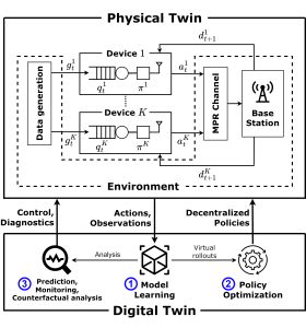
Integrated sensing and communications (ISAC), a key enabling technology for 6G systems, leverages shared radio resources and hardware to realize the functions of sensing and communication. As an example of an application that can benefit from ISAC, consider the inter-vehicle communication scenario in Fig. 1. In it, a car wishes to send a message to a second car, while also enabling the latter to detect the presence of a possible target, e.g., of a pedestrian. While conventional systems would use two separate radio resources for data transmission and radar detection, ISAC solutions reuse the same transmitted waveform for the dual role of carrier of digital information and radar signal [1]. A natural radio interface to serve this dual function is impulse radio (IR), also known as ultrawideband (UWB). In fact, IR encodes information in the timing of pulses, which can in turn be repurposed for radar detection [2].

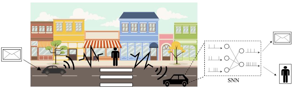
Fig. 1. Illustration of a neuromorphic ISAC system, in which the same IR (or UWB) signal is used for transmission and radar detection of the presence of a target. The key novel element is the use of neuromorphic computing at the ISAC receiver to simultaneously demodulate digital data and provide an online estimate of the presence or absence of the radar target.

Neuromorphic sensing and computing are emerging as alternative, brain-inspired, paradigms for efficient data collection and semantic signal processing [3]. The main features of this technology are energy efficiency, native event-driven processing of time-varying semantic sources, spike-based computing, and always-on on-hardware adaptation [4]. Neuromorphic processors, also known as spiking neural networks (SNNs), are networks of dynamic spiking neurons that mimic the operation of biological neurons. When implemented on specialized — digital or mixed analog-digital — hardware or on tailored FPGA configurations, SNNs have minimal idle and operating energy cost, and consume as little as a few picojoules per spike [5].

The integration of IR and neuromorphic computing was investigated in our recent works [6, 7], which proposed an end-to-end neuromorphic architecture for remote inference that replaces traditional digital blocks with SNNs as encoder and decoder.

Our work

With the aim of reducing energy consumption and facilitating online and always-on operation on specialized hardware, as illustrated in Fig. 1, we propose to leverage the synergy between IR transmission and neuromorphic computing to realize efficient ISAC systems. The neuromorphic ISAC (N-ISAC) receiver is able to leverage spiking neural network (SNN)-based processing to demodulate digital information and detect the radar signal.

As illustrated in Fig. 2, we consider an ISAC system in which digital communication and radar sensing leverage the same IR transmitted signal. In order to efficiently and simultaneously decode the digital data and detect the possible presence of a target at a known delay cell, the receiver processes the received signal via an SNN. Technical details can be found in our paper at this link.

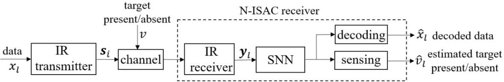
Fig. 2. N-ISAC: Digital data is transmitted by an IR transmitter via pulse-position modulation (PPM); while the receiver simultaneously decodes digital data, and performs radar detection by means of an SNN, which can be efficiently implemented on neuromorphic hardware.

Result

We compare the proposed N-ISAC system with a conventional separate sensing and communications (SSAC) scheme, which divides the transmission slots into slots used for transmission and slots used for sensing. For SSAC, two SNNs are implemented at the receiver, one performing data decoding for the transmission slots, and the other responsible for radar sensing in the sensing slots.

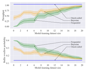
To evaluate the performance of our system, we adopt the following performance metrics for data transmission and radar sensing: 1) Normalized test throughput, i.e., the ratio of the average number of correctly decoded bits over the total number of time slots; 2) Radar test detection error, i.e., the probability that the sensing decision is not correctly taken upon processing all time slots.

In Fig. 3, we demonstrate the normalized test throughput versus the radar test detection error for ISAC and SSAC. For the ISAC scheme, we vary a hyperparameter β dictating the relative weight in the design criterion in favor of communications; for SSAC we vary the fraction α of slots allocated to communications. As β increases, more priority is given by ISAC to communication over radar detection; and, similarly, as α increases, SSAC assigns more slots to communications. The performance of ISAC with an SNN having 10 hidden neurons is essentially independent of β for any 0.25< β <0.75. A first observation is that, for SSAC, there is a trade-off between communication and sensing performance levels caused by the slot allocation. A similar trade-off is also observed for ISAC when using an SNN with 6 hidden neurons. This is due to the limited capacity of the shared common hidden layer of the SNN. In contrast, when 10 hidden neurons are available at the SNN, ISAC is seen to optimize both data decoding and target sensing performance, obtaining significant gains over SSAC.

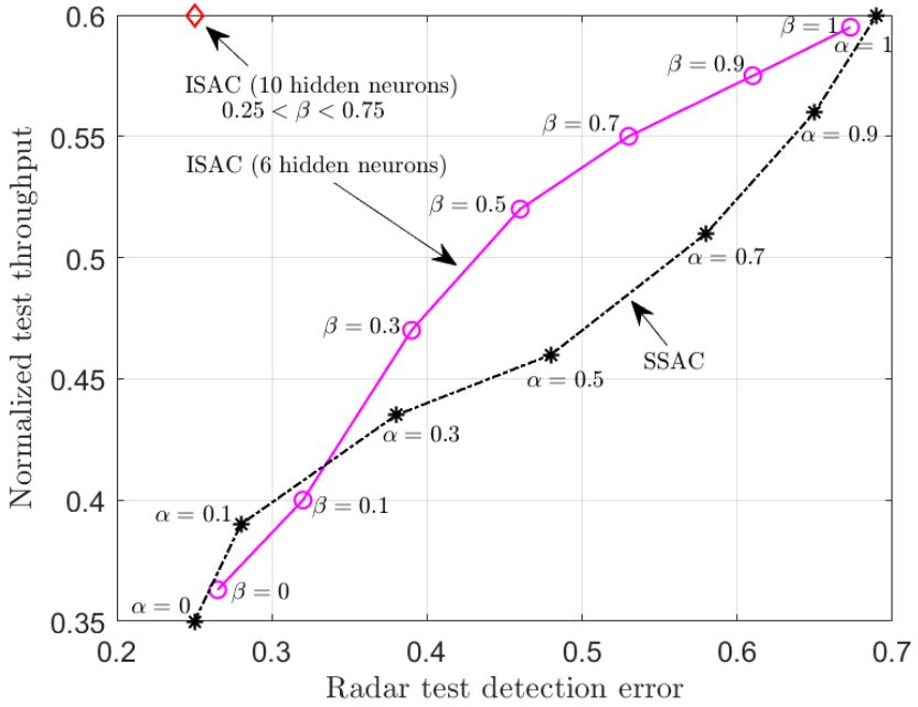
Fig. 3. Normalized test throughput versus radar test detection error for ISAC and SSAC.

Fig. 4 illustrates how the SNN receiver can leverage the temporal sparsity of the IR signals to enhance energy efficiency. In this regard, we recall that energy consumption in an SNN is essentially proportional to the number of spikes produced by the SNN, given extremely low idle energy of neuromorphic chips [8]. The top panel shows the transmitted IR signal consisting of two frames of transmitted signals, separated by an idle frame of duration of 20 slots. We observe that in the idle frame, the spike count is significantly reduced, showing that the neuromorphic receiver can adjust its energy consumption to the activity level of the transmitter.

Fig. 4. Top: Transmitted signal consisting of two frames in which the transmitter is active separated by an idle frame. Bottom: Corresponding spike count for the SNN.

References

[1] S. Jeong, O. Simeone, A. Haimovich, and J. Kang, “Beamforming design for joint localization and data transmission in distributed antenna system,” IEEE Transactions on Vehicular Technology, vol. 64, no. 1, pp. 62–76, 2014.

[2] A. Nezirovic, A. G. Yarovoy, and L. P. Ligthart, “Signal processing for improved detection of trapped victims using UWB radar,” IEEE Transactions on Geoscience and Remote Sensing, vol. 48, no. 4, pp. 2005–2014, 2009.

[3] A. Mehonic and A. J. Kenyon, “Brain-inspired computing needs a master plan,” Nature, vol. 604, no. 7905, pp. 255–260, 2022.

[4] M . Davies, A. Wild, G. Orchard, Y. Sandamirskaya, G. A. F. Guerra, P. Joshi, P. Plank, and S. R. Risbud, “Advancing neuromorphic computing with Loihi: a survey of results and outlook,” Proceedings of the IEEE, vol. 109, no. 5, pp. 911–934, 2021.

[5] B. Rajendran, A. Sebastian, M. Schmuker, N. Srinivasa, and E. Eleftheriou, “Low-power neuromorphic hardware for signal processing applications: a review of architectural and system-level design approaches,” IEEE Signal Processing Magazine, vol. 36, no. 6, pp. 97–110, 2019.

[6] N. Skatchkovsky, H. Jang, and O. Simeone, “End-to-end learning of neuromorphic wireless systems for low-power edge artificial intelligence,” in Proc. Asilomar Conference on Signals, Systems, and Computers, pp. 166–173, 2020.

[7] J. Chen, N. Skatchkovsky, and O. Simeone, “Neuromorphic wireless cognition: event-driven semantic communications for remote inference,” arXiv preprint arXiv:2206.06047, 2022.

[8] M . Davies, N. Srinivasa, T.-H. Lin, G. Chinya, Y. Cao, S. H. Choday, G. Dimou, P. Joshi, N. Imam, S. Jain et al., “Loihi: A neuromorphic manycore processor with on-chip learning,” IEEE Micro, vol. 38, no. 1, pp. 82–99, 2018.

Whilst the true impact of quantum computers is anybody’s guess, there seems to be some consensus on the advantages offered by near-term devices in modeling more complex probability distributions. These distributions can be used to model complex particle interactions, e.g., in quantum chemistry, or, as we will see next, to train principled machine learning models – in this case, binary Bayesian neural networks – and enable fast adaptation to new learning tasks from few training examples.

Fig. 1. (left) A binary Bayesian neural network, i.e., a neural network with stochastic binary weights, is trained to carry out a learning task. (right) The probability distribution of the binary weights of the neural network is modelled by a Born machine, i.e., by a parametric quantum circuit (PQC), leveraging the PQC’s capacity to model complex distributions [1].

Setting

In our latest work, accepted for presentation at the IEEE MLSP, we are interested in training Bayesian binary neural networks, i.e., classical neural networks with stochastic binary weights, in a sample-efficient manner by means of meta-learning, as illustrated in Fig. 1. The key idea of this work is to model the distribution of the binary weights via a Born machine, i.e., via a probabilistic parametric quantum circuit (PQC), due to the capacity of PQCs to efficiently implement complex probability distributions [1]-[4]. We propose a novel method that integrates meta-learning with the gradient-based optimization of quantum Born machines [3], with the aim of speeding up adaptation to new learning tasks from few examples.

Born Machines

A Born machine produces random binary strings  , where    denotes the total number of model parameters, by measuring the output of a PQC  defined by parameters  .

Fig. 2. Hardware-efficient ansatz for a Born machine. All qubits are initialized in the ground state. The rotations are parametrized by the entries of the variational vector.

As illustrated in Fig. 2, the PQC takes the initial state    of n qubits as an input, and operates on it via a sequence of unitary gates described by a unitary matrix   . This operation outputs the final quantum state

which is measured in the computational basis to produce a random binary string . Note that each basis vector of the computational basis corresponds to one of all the possible 2^n patterns of model parameters  .

The PQC can be implemented using a hardware-efficient ansatz [2], in which a layer of one-qubit unitary gates, parametrized by vector , is followed by a layer of fixed, entangling, two-qubit gates. This pattern can be repeated any number of times, building a progressively deeper circuit. Another option is using the mean-field ansatz that does not use entangling gates, and only relies on one-qubit gates.

By Born’s rule (hence the name of the circuit), the probability distribution of the output model parameter vector is given by

Importantly, Born machines only provide samples, while the actual distribution above can only be estimated by averaging multiple measurements of the PQC’s outputs. Therefore, Born machines model implicit distributions, and only define a stochastic procedure that directly generates samples.

Some Results

Fig. 3 illustrate the results in terms of the prediction root mean squared error (RMSE) as a function of the number of meta-training iterations. By comparison with conventional per-task learning, the figure illustrates the capacity of both joint learning and meta-learning to transfer knowledge from the meta-training to the meta-test task, with hardware-efficient (HE) and mean-field (MF) quantum meta-learning clearly outperforming joint learning. For example, HE meta-learning requires around 150 meta-training iterations to achieve the same RMSE ideal per-task training, whilst joint-learning requires more than 200 to achieve comparable performance. The HE ansatz performs best, due to the use of entangling unitaries; however, the MF ansatz approaches the minimal RMSE after 230 iterations. The classical solution based on MF Bernoulli does not achieve lower RMSE than the quantum-aided meta-learning schemes, even with joint learning.

Fig. 3. Average RMSE for a new, meta-test, task as a function of the number of meta-training iterations. The results are averaged over 5 independent trials.

Please see the paper for a more detailed exposition, available here.

References

[1] Arute, F., Arya, K., Babbush, R., Bacon, D., Bardin, J.C., Barends, R., Biswas, R., Boixo, S., Brandao, F.G., Buell, D.A., et al.: Quantum supremacy using a programmable superconducting processor. Nature 574(7779), 505–510 (2019)
[2] Kandala, A., Mezzacapo, A., Temme, K., Takita, M., Brink, M., Chow, J.M., Gambetta, J.M.: Hardware-efficient variational quantum eigensolver for small molecules and quantum magnets. Nature 549(7671), 242–246 (2017)
[3] Liu, J.G., Wang, L.: Differentiable learning of quantum circuit Born machines. Physical Review A 98(6), 062324 (2018)
[4] Sweke, R., Seifert, J.P., Hangleiter, D., Eisert, J.: On the quantum versus classical learnability of discrete distributions. Quantum 5, 417 (2021)

In 1959 Richard Feynman gave an after-dinner talk at an American Physics Society meeting in Pasadena entitled “There’s Plenty of Room at the Bottom”,  crediting Edward Fredkin for inspiration.  In his talk, the transcription of which would later become a landmark paper in quantum computation and simulation [1], he takes some existing ideas — computation is a physical process, perhaps even a quantum mechanical one — and makes a particularly famous statement:

”I’m not happy with all the analyses that go with just classical theory, because Nature isn’t classical, dammit, and if you want to make a simulation of Nature, you’d better make it quantum mechanical, and by golly it’s a wonderful problem!”

But how can we simulate the quantum mechanical nature of Nature? This new kind of machine would become the quantum computer, and from then on, quantum computing has been on a journey with many ups and downs. Nowadays, excitement seems to be in the air again as quantum machine learning, a hybrid research discipline that combines machine learning and quantum computing, has emerged as a potential practical use of quantum hardware. Generally, quantum machine learning methods apply classical optimization routines to select parameters that define the operation of a quantum circuit. Alternative approaches, which may be more promising in the short term, involve hybrid quantum-classical models, where classical computation, e.g., for feature extraction, is combined with quantum parametric circuits [2].

Our Work

In our latest work, published in the IEEE Signal Processing Letters, we focus on the hybrid classical-quantum two-layer architecture illustrated in Fig. 1.

Fig. 1. In the studied hybrid classical-quantum classifier, a quantum hidden layer, fed via amplitude encoding and consisting of quantum generalized linear models (QGLMs), is followed by a classical combining output layer with a single classical GLM (CGLM) neuron. All weights and activations are binary.

In it, a first layer of quantum generalized linear models (QGLMs) is followed by a second classical combining layer. The input to the first, hidden, layer is obtained via amplitude encoding (see, e.g., [3]). Several implementations of QGLM neurons have been proposed in the literature using different quantum circuits. Given a binary input sample  and an N-dimensional vector of binary weights, the main goal of these circuits is to produce a stochastic binary output with probabilities which are a function of the inner product

between the input state and the amplitude-encoded binary weight vector

Different solutions, along with the resulting QGLM neuron’s response functions are given in the paper. For this hybrid model, we introduced a stochastic variational optimization (SVO) approach [4] that enables the joint training of quantum and classical layers via stochastic gradient descent. The proposed SVO-based training strategy operates in a relaxed continuous space of variational classical parameters.

Some Results

We show the classification accuracy, which is defined as the ratio of the number of accurate predictions over the total number of predictions made by the model, in Fig. 2 as a function of the training iterations.

Fig. 2. Classification accuracy as a function of the training iteration for the benchmark sign-flips scheme [5] and the proposed SVO-based procedure for the BAS data set. The results are averaged over 5 independent trials.

The proposed SVO scheme is seen to achieve high classification accuracy for all of the considered response functions. In particular, the QGLM using the Quadratic (Q) response function yields fastest convergence and achieves the best performance. Due to the additional bias terms resulting from the swap test routine, the QGLMs relying on the Biased quadratic (BQ) and Biased centered quadratic (BCQ) response functions are slower to learn, but ultimately converge after around 3000 training iterations.

Please see the paper for a more extensive presentation, available here

Code, alongside a tutorial, are available here

References

[1] R. P. Feynman et al., “Simulating physics with computers,” Int. j. Theor. phys, vol. 21, no. 6/7, 1982.
[2] A. Mari, T. R. Bromley, J. Izaac, M. Schuld, and N. Killoran, “Transfer learning in hybrid classical-quantum neural networks,” Quantum, vol. 4, p. 340, 2020.
[3] M. Schuld and F. Petruccione, Machine Learning with Quantum Computers. Springer, 2021.
[4] T. Bird, J. Kunze, and D. Barber, “Stochastic variational optimization,” arXiv preprint arXiv:1809.04855, 2018.
[5] F. Tacchino, C. Macchiavello, D. Gerace, and D. Bajoni, “An artificial neuron implemented on an actual quantum processor,” npj Quantum Information, vol. 5, no. 1, pp. 1–8, 2019

The overall predictive uncertainty of a trained predictor comprises of two main contributions: the aleatoric uncertainty arising due to inherent randomness in the data generation process and the epistemic uncertainty resulting due to limitations of available training data. While the epistemic uncertainty, also called minimum excess risk, can be made to vanish with increasing training data, the aleatoric uncertainty is independent of the data. In our recent work accepted to AISTATS 2022, we provide an information-theoretic quantification of the epistemic uncertainty arising in the broad framework of Bayesian meta-learning.

Problem Formulation

In conventional Bayesian learning, the model parameter   that describes the data generating distribution is assumed to be random and is endowed with a prior distribution. This distribution is conventionally chosen based on prior knowledge about the problem. In contrast,  Bayesian meta-learning (see Fig. 1 below) aims to automatically infer this prior distribution by observing data from several related tasks. The statistical relationship among the tasks is accounted for via a global latent hyperparameter .  Specifically, the model parameter for each observed task  is drawn according to a shared prior distribution   with shared global hyperparameter . Following the Bayesian formalism, the hyperparameter is assumed to be random and distributed according to a hyper-prior distribution .

Figure 1: Bayesian meta-learning decision problem

The data from the observed related tasks, collectively called meta-training data, is used to reduce the expected loss incurred on a test task. The test task is modelled as generated by an independent model parameter  with the same shared hyperparameter. This model parameter underlies the generation of a test task training data, used to infer the task-specific model parameter, as well as a test data sample from the test task. The Bayesian meta-learning decision problem is to predict the label corresponding to test input feature of the test task, after observing the meta-training data and the training data of the test task.

A meta-learning decision rule    thus maps the meta-training data, the test task training data and test input feature to an action space.  The Bayesian meta-risk can be defined as the minimum expected loss incurred over all meta-learning decision rules, i.e., .  In the genie-aided case when the model parameter and hyper-parameter are known, the genie-aided Bayesian risk is defined as  . The epistemic uncertainty, or minimum excess risk, corresponds to the difference between the Bayesian meta-risk and Genie-aided meta-risk as  .

Main Result

Our main result shows that under the log-loss, the minimum excess meta-risk can be exactly characterized using the conditional mutual information

where H(A|B)  denotes the conditional entropy of A given B and  I(A;B|C) denotes the conditional mutual information between A and B given C.  This in turn implies that

More importantly, we show that the epistemic uncertainty is contributed by two levels of uncertainties – model parameter level and hyperparameter level as

which scales in the order of 1/Nm+1/m, and vanishes as both the number of observed tasks and per-task data samples go to infinity. The behavior of the bounds is illustrated for the problem of meta-learning the Bayesian neural network prior for regression tasks in the figure below.

Figure 2: Performance of MEMR and derived upper bounds as a function of number of tasks and per-task data samples

Problem

An essential property of any wireless channel is the fact that it is a shared medium, much like the air through which sound propagates is shared among the participants of a conversation. As a result, communication engineers must deal with the resulting interference,  which may substantially limit the reliability and the achievable rates in a wireless communication system. A proven remedy is to adapt the transmission power to current channel conditions, which was successfully addressed by the data-driven methodology introduced in [1] in which the power control policy is parametrized by a random edge graph neural network (REGNN).

In our recent work to be presented at SPAWC 2021, we focus on the higher-level problem of facilitating adaptation of the power control policy. We consider the case where the topology of the network varies across periods of operation of the system, with each period being in turn characterized by time-varying channel conditions. In order to facilitate fast adaptation of the power control policy — in terms of data and iteration requirements — we integrate meta-learning with REGNN training.

Meta-learning Solution

Our meta-learning solution leverages channel state information (CSI) data from a number of previous periods to optimize an adaptation procedure that facilitates fast adaptation on a new topology to be encountered in a future period. We specifically adopt first-order meta-learning methods, namely first-order model agnostic meta-learning (FOMAML) [2] and REPTILE [3] that parametrize the adaptation procedure via its initialization within each period. While GNNs are known to be robust to changes in the topology, the proposed integration of meta-learning and REGNNs is shown to offer significant improvements in terms of sample and iteration efficiency.

Fig 1. Sum rate as a function of the number of samples used for adaptation, for a network with dynamic size.

Some Results

The achievable sum rate with respect to the number of CSI samples used for adaptation is illustrated in Fig. 1 for a network in which the number of transmitters and receivers changes in each period. Meta-learning, via both FOMAML and REPTILE, is seen to adapt quickly to the new topology, outperforming conventional REGNN, even when allowing for fine-tuning of the later. This significant improvement can be attributed to the variability of the topologies observed across periods in the considered scenario, which makes the joint training approach in [1] ineffective. That said, when the number of samples for adaptation is sufficiently large, conventional REGNN training as in [1] outperforms meta-learning, as the initialization obtained by meta-learning induces a more substantial bias than joint training due to the mismatch in the conditions assumed for the updates on meta-training and meta-testing tasks (i.e., the different number of samples used for meta-training and adaptation).

Please see the paper for more results and a more extensive analysis, which is available here

[1] M. Eisen and A. Ribeiro, “Optimal wireless resource allocation with random edge graph neural networks,”IEEE Transactionson Signal Processing, vol. 68, pp. 2977–2991, April, 2020.

[2] C. Finn, P. Abbeel, and S. Levine, “Model-agnostic meta-learning for fast adaptation of deep networks,” inProc. InternationalConference on Machine Learning (PMLR). Sydney, 6–11 August, 2017, pp. 1126–1135.

[3] A. Nichol, J. Achiam, and J. Schulman, “On first-order meta-learning algorithms,”arXiv preprint arXiv:1803.02999, 2018.