Category: Machine Learning

Life-long brain-inspired learning that knows what it does not know

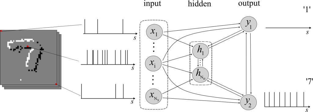
An emerging research topic in artificial intelligence (AI) consists in designing systems that take inspiration from biological brains. This is notably driven by the fact that, although most AI algorithms become more and more efficient (for instance, for image generation), this comes at a cost. Indeed, with architectures constantly growing in size, training a single large neural network today consumes a prohibitive amount of energy. Despite consuming only about 12W, human brains exhibit impressive capabilities, such as life-long learning.

By taking a Bayesian perspective, we demonstrate in our latest work how biologically inspired spiking neural networks (SNNs) can exhibit learning mechanisms similar to those applied in brains, which allow them to perform continual learning. As we will see, the technique also solves a key challenge in deep learning, that is, to obtain well calibrated solutions in the face of previously unseen data.


Our work

Bayesian Learning

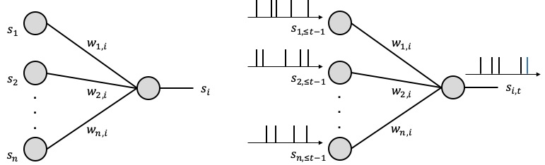
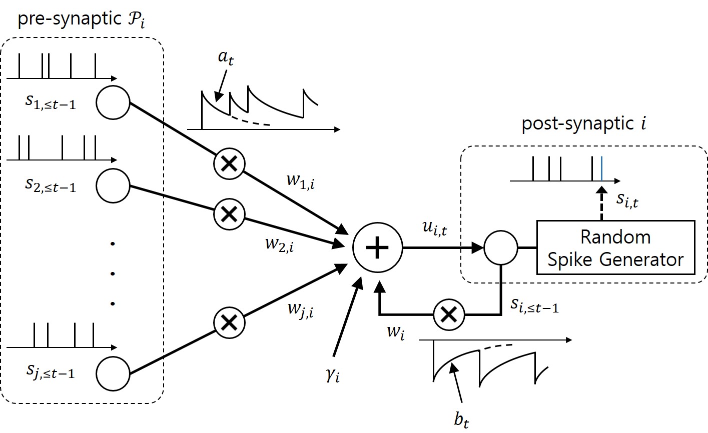
As seen in Fig. 1, we propose to equip each synaptic weight in the SNN with a probability distribution. The distribution captures the epistemic uncertainty induced by the lack of knowledge of the true distribution of the data. This is done by assigning probabilities to model parameters that fit equally well the data, while also being consistent with prior knowledge. As a consequence, Bayesian learning is known to produce better calibrated decisions, i.e., decisions whose associated confidence better reflects the actual accuracy of the decision.

This contrasts with frequentist learning, in which the vector of synaptic weights is optimized by minimizing a training loss. The training loss is adopted as a proxy for the population loss, i.e., for the loss averaged over the true, unknown, distribution of the data. Therefore, frequentist learning disregards the inherent uncertainty caused by the availability of limited training data, which causes the training loss to be a potentially inaccurate estimate of the population loss. As a result, frequentist learning is known to potentially yield poorly calibrated, and overconfident decisions for ANNs.

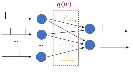
Figure 1: Illustration of Bayesian learning in an SNN: In a Bayesian SNN, the synaptic weights are assigned a joint distribution, often simplified as a product distribution across weights.

We consider both real-valued (with possibly limited resolution, as dictated by deployment on neuromorphic hardware) and binary-valued synapses, parametrised by Gaussian and Bernoulli distributions, respectively. The advantages of models with binary-valued synapses, i.e., binary SNNs, include a reduced complexity for the computation of the membrane potential. Furthermore, binary SNNs are particularly well suited for implementations on chips with nanoscale components that provide discrete conductance levels for the synapses.


Continual Learning

In addition to uncertainty quantification, we apply the proposed solution to continual learning, as illustrated in Fig. 2. In continual learning, the system is sequentially presented several datasets corresponding to distinct, but related, learning tasks, where each task is selected, possibly with replacement, from a pool of tasks, and its identity is unknown to the system. Its goal is to learn to make predictions that generalize well each new task, while causing minimal loss of accuracy on previous tasks.

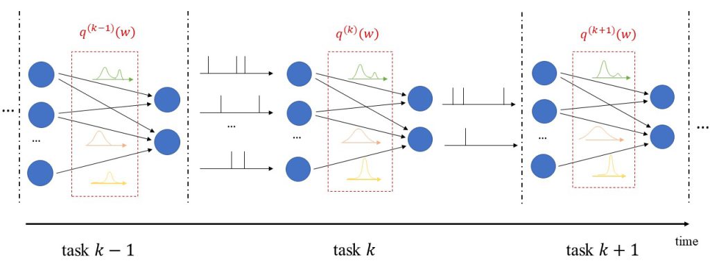
Figure 2: Illustration of Bayesian continual learning: the system is successively presented with similar, but different, tasks. Bayesian learning allows the model to retain information about previously learned information.

Many existing works on continual learning draw their inspiration from the mechanisms underlying the capability of biological brains to carry out life-long learning. Learning is believed to be achieved in biological systems by modulating the strength of synaptic links. In this process, a variety of mechanisms are at work to establish short-to intermediate-term and long-term memory for the acquisition of new information over time. These mechanisms operate at different time and spatial scales.


Biological Principles of Learning

One of the best understood mechanisms, long-term potentiation, contributes to the management of long-term memory through the consolidation of synaptic connections. Once established, these are rendered resistant to disruption by changing their capacity to change via metaplasticity. As a related mechanism, return to a base state is ensured after exposition to small, noisy changes by heterosynaptic plasticity, which plays a key role in ensuring the stability of neural systems. Neuromodulation operates at the scale of neural populations to respond to particular events registered by the brain. Finally, episodic replay plays a key role in the maintenance of long-term memory, by allowing biological brains to re-activate signals seen during previous active periods when inactive (i.e., sleeping).

In this work, we demonstrate how the continual learning rule we obtain exhibits some of these mechanisms. In particular, synaptic consolidation and metaplasticity for each synapse can be modeled by a precision parameter. A larger precision reduces the step size of the synaptic weight updates. During learning, the precision is increased to the degree that depends on the relevance of each synapse as measured by the estimated Fisher information matrix for the current mini-batch of examples.

Heterosynaptic plasticity, which drives the updates towards previously learned and resting states to prevent catastrophic forgetting, is obtained from first principles via an information risk minimization formulation with a Kullback-Leibler regularization term. This mechanism drives the updates of the precision and mean parameter towards the corresponding parameters of the variational posterior obtained at the previous task.

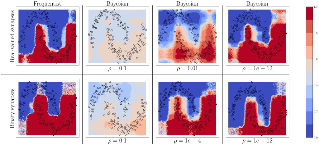
Figure 3: Predictive probabilities evaluated on the two-moons dataset after training for Bayesian learning. Top row: Real-valued synapses; Bottom row: Binary synapses.

Results

We start by considering the two-moons dataset shown in Fig. 3. Triangles indicate training points for a class “0’’, while circles indicate training points for a class “1”. The color intensity represents the predictive probabilities for frequentist learning and for Bayesian learning: the more intense the color, the higher the prediction confidence determined by the model. Bayesian learning is observed to provide better calibrated predictions, that are more uncertain outside the input regions covered by training data points. As can be seen, confidence for the Bayesian models can be mitigated by a parameter, as precised in the full text.

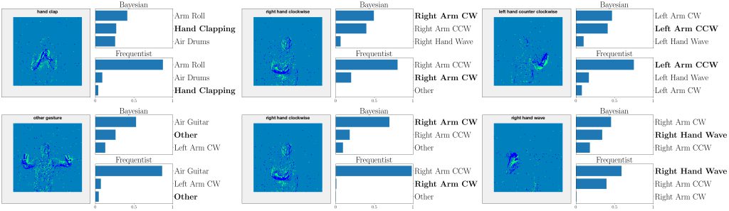
Figure 4: Top three classes predicted by both Bayesian and frequentist models on selected examples from the DVS-Gestures dataset. Top: real-valued synapses. Bottom: binary synapses. The correct class is indicated in bold font.

This point is further illustrated in Fig. 4 by showing the three largest probabilities assigned by the different models on selected examples from DVS-Gestures dataset, considering real-valued synapses in the top row and binary synapses in the bottom row. In the left column, we observe that, when both models predict the wrong class, Bayesian SNNs tend to do so with a lower level of certainty, and typically rank the correct class higher than their frequentist counterparts. Specifically, in the examples shown, Bayesian models with both real-valued and binary synapses rank the correct class second, while the frequentist models rank it third. Furthermore, as seen in the middle column, in a number of cases, the Bayesian models manage to predict the correct class, while the frequentist models predict a wrong class with high certainty. In the right column, we show that even when frequentist models predict the correct class and Bayesian models fail to do so, they still assign lower probabilities (i.e., <50%) to the predicted class.

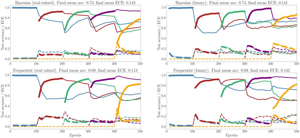
Figure 5: Evolution of the average test accuracies and ECE on all tasks of the split-MNIST-DVS across training epochs, with Gaussian and Bernoulli variational posteriors, and frequentist schemes for both real-valued and binary synapses. Continuous lines: test accuracy, dotted lines: ECE, bold: current task. Blue: {0, 1}; Red: {2, 3}; Green: {4, 5}; Purple:{6, 7}; Yellow: {8, 9}.

Finally, we show results for continual learning on the MNIST-DVS dataset in Fig. 5. We show the evolution of the test accuracy and expected calibration error (ECE) on all tasks, represented with lines of different colors, during training. The performance on the current task is shown as a thicker line. We consider frequentist and Bayesian learning, with both real-valued and binary synapses. With Bayesian learning, the test accuracy on previous tasks does not decrease excessively when learning a new task, which shows the capacity of the technique to tackle catastrophic forgetting. Also, the ECE across all tasks is seen to remain more stable for Bayesian learning as compared to the frequentist benchmarks. For both real-valued and binary synapses, the final average accuracy and ECE across all tasks show the superiority of Bayesian over frequentist learning.

More details can be found in the full text at this link.

“Hyper-Learning” How to Transfer from Uplink to Downlink for Massive MIMO

Problem

Most cellular deployments rely on frequency division duplex (FDD) due to its lower latency and greater coverage potential. In FDD, uplink and downlink channels use different carrier frequencies. Therefore, as illustrated in Fig. 1, with FDD, downlink channel state information (CSI) cannot be directly obtained from uplink pilots due to a lack of full reciprocity between uplink and downlink channels.

Fig.1 FDD massive MIMO system over multipath channels with partial reciprocity

The conventional solution to this problem is to leverage downlink training and feedback from the devices. This, however, generally causes a prohibitively large downlink and uplink overhead in massive multiple-input multiple-output (MIMO) systems owing to the need to transmit a pilot sequences of length proportional to the number of antennas.

State-of-the-art recent proposals to address the inefficiencies of this conventional solutions adopt machine learning (ML) tools. The use of ML is justified by the technical challenges arising from the lack of efficient optimal model-based methods.

In our recent work to be presented at SPAWC 2021, we contribute to this line of work by introducing a new ML-based solution that improves over the state of the art by leveraging partial channel reciprocity and the tool of hypernetworks.

Our approach


Fig. 2 The proposed HyperRNN architecture for end-to-end channel estimation based on temporal correlations and partial reciprocity

In this work, we propose a novel end-to-end architecture — HyperRNN — illustrated in Fig. 2. The main innovation of the approach is that simultaneously transmitted pilot symbols in the uplink, across multiple time slots, are leveraged to automatically extract long-term reciprocal channel features (see Fig. 1) via a hypernetwork that determines the weight of the downlink CSI estimation or beamforming network. Importantly, the long-term features implicitly underlie the discriminative mapping implemented by the hypernetwork between uplink pilots and downlink CSI estimation network, rather than estimated explicitly. The second main innovation is to incorporate recurrent neural networks (RNNs), in lieu of (feedforward) deep neural networks (DNNs) for both uplink and downlink processing in order to leverage the temporal correlation of the fading amplitudes.

Results

We compare the the normalized mean square error (NMSE) performance of our proposed HyperRNN and an earlier work based on end-to-end training procedure, downlink-based DNN (DL-DNN), which encompasses downlink pilot training, distributed quantization for the uplink and downlink channel estimation. Simulations are performed over the spatial channel model (SCM) standardized in 3GPP Release 16. Fig. 3 demonstrates the NMSE of the proposed HyperRNN and of the benchmark DL-DNN for channel estimation as a function of the number of paths. Larger performance gains can be achieved when the channel has a lower number of paths. In fact, in this regime, the invariant of the long-term features of the channel defines a low-rank structure of the channel that can be leveraged by the hypernetwork.

Fig. 3 NMSE of the HyperRNN and DL-DNN over frequency-flat fading channels having different number of paths for an FDD system

Full paper can be found here.

Privacy in Wireless Federated Learning is Free

–when the SNR is small enough

Problem Description 

Federated Learning (FL) refers to distributed protocols that avoid direct raw data exchange among the participating devices while training for a common learning task. This way, FL can potentially reduce the information on the local data sets that is leaked via communications. Nevertheless, the model updates shared by the devices may still reveal information about local data. For example, a malicious server could potentially infer the presence of an individual data sample from a learnt model by membership inference attack or model inversion attack. 

Differential privacy (DP) quantifies information leaked about individual data points by measuring the sensitivity of the disclosed statistics to changes in the input data set at a single data point. DP can be guaranteed by introducing a level of uncertainty into the released model that is sufficient to mask the contribution of any individual data point. The most typical approach is to add random perturbations, e.g., Gaussian. This suggests that,  when FL is implemented in wireless systems, the channel noise can directly act as a privacy-inducing mechanism. 

Suggested Solution 

In recent work, we have designed differentially private wireless distributed gradient descent via the direct, uncoded, transmission of gradients from devices to edge server. The channel noise is utilized as a privacy preserving mechanism and dynamic power control is separately optimized for orthogonal multiple access  (OMA) and non-orthogonal multiple access  (NOMA) protocols with the goal of minimizing the learning optimality gap under privacy and power constraints across a given number of communication blocks.  Our recent work to appear in IEEE Journal on Selected Areas in Communications tackles this problem. One of our main results shows that, as long as the privacy constraint level, measured via DP, is below a threshold that decreases with the signal-to-noise ratio (SNR), uncoded transmission achieves privacy “for free”, i.e., without affecting the learning performance. As our analysis demonstrates, channel noise added in the first iterations tends to impact convergence less significantly than the noise added in later iterations, whereas the privacy level depends on a weighted sum of the inverse noise power across the iteration. These properties, captured by compact analytical expressions derived in this paper, are leveraged for adaptive power allocation, yielding significant performance gains over standard static power allocation. 

Some Results 

The performance is first evaluated by using randomly generated synthetic dataset. In the considered range of DP level,  as illustrated in the figure below, NOMA with either adaptive or static power allocation (PA) achieves better performance than OMA. Furthermore, the proposed adaptive PA obtains a significant performance gain over static PA under stringent DP constraints, while the performance advantage of adaptive PA decreases as the DP constraint is relaxed. The figure also shows the threshold values of DP level beyond which the privacy “for free”.  

The performance is also evaluated by MNIST data set as summarized in the last figure. With conventional static PA, the increasing communication budget is seen to largely degrade performance. This is because more communication blocks may cause an increase in privacy loss. In contrast, adaptive PA is able to properly allocate power across the communication blocks thereby achieves a lower training loss.

Federated Neuromorphic Computing

Problem
Training state-of-the-art Artificial Neural Network (ANN) models requires distributed computing on large mixed CPU-GPU clusters, typically over many days or weeks, at the expense of massive memory, time, and energy resources, and potentially of privacy violations. Alternative solutions for low-power machine learning on resource-constrained devices have been recently the focus of intense research. In our recently accepted paper at ICASSP 2020, we study the convergence of two such recent lines of inquiries.

On the one hand, Spiking Neural Networks (SNNs) are biologically inspired neural networks in which neurons are dynamic elements processing and communicating via sparse spiking signals over time, rather than via real numbers, enabling the native processing of time-encoded data, e.g., from DVS cameras. They can be implemented on dedicated hardware, offering energy consumptions as low as a few picojoules per spike. A more thorough introduction to probabilistic SNNs can be found in this previous blog post.

On the other hand, Federated Learning (FL) allows devices to carry out collaborative learning without exchanging local data. This makes it possible to train more effective machine learning models by benefiting from data at multiple devices with limited privacy concerns. FL requires devices to periodically exchange information about their local model parameters through a parameter server. It has become de-facto standard for training ANNs over large numbers of distributed devices.

System model

Figure 1 Federated Learning (FL) model under study: Mobile devices collaboratively train on-device SNNs based on different, heterogeneous, and generally unbalanced local data sets, by communicating through a base station (BS).

In our work, as seen in Figure 1, we consider a distributed edge computing architecture in which N mobile devices communicate through a Base Station (BS) in order to perform the collaborative training of local SNN models via FL. Each device holds a different local data set. The goal of FL is to train a common SNN-based model without direct exchange of the data from the local data sets.

FL proceeds in an iterative fashion across T global time-steps. To elaborate, at each global time-step, the devices refine their local model, based on their local datasets. Every τ iterations, they will also transmit their updated local model parameters to the BS, which will in turn compute a centralized averaged parameter and send it back to the devices. This global averaged parameter will be used at the beginning of the next iteration.

An SNN is a network of spiking neurons connected via an arbitrary directed graph, possibly with cycles (see Figure 2). SNNs process information through time, based on a local clock. At each local algorithmic time-step, each neuron receives the signals emitted by the subset of neurons connected to it through directed links, known as synapses. Neurons in the network will then output a binary signal, either ‘0’ or ‘1’. The instantaneous spiking probability of a neuron is determined by its past spiking behaviour and the previous spikes of its pre-synaptic neurons. SNNs are trained over sequences of S local algorithmic time-steps, made of D examples of length S’. In an image classification task, an example could be an image encoded as a binary signal.

Figure 2 Example of an internal architecture for an on-device SNN.

In FL-SNN, we cooperatively train distributed on-device SNNs thanks to Federated Learning. To that end, we derived a novel algorithm, for which the time scales involved are summarized in Figure 3. Each global algorithmic iteration t corresponds to Δs local SNN time-steps, and the total number S of SNN local algorithmic time steps and the number T of global algorithmic time steps during the training procedure are hence related as S = DS’ = T∆s.

Figure 3 Illustration of the time scales involved in the cooperative training of SNNs via FL for τ = 3 and ∆s = 4.

Experiments

We consider a classification task based on the MNIST-DVS dataset. The training dataset is composed of 900 examples per class and the test dataset is composed of 100 samples per class. We consider 2 devices which have access to disjoint subsets of the training dataset. In order to validate the advantages of FL, we assume that the first device has only samples from class ‘1’ and the second only from class ‘7’. We train over D = 400 randomly selected examples from the local data sets, which results in S = DS’ = 32,000 local time-steps.

As a baseline, we consider the test loss at convergence for the separate training of the two SNNs. In Figure 4, we plot the local test loss normalized by the mentioned baseline as a function of the global algorithmic time. A larger communication period τ is seen to impair the learning capabilities of the SNNs, yielding a larger final value of the loss. In fact, for τ = 400, after a number of local iterations without communication, the individual devices are not able to make use of their data to improve performance.

Figure 4 Evolution of the mean test loss during training for different values of the communication period τ. Shaded areas represent standard deviations over 3 trials

One of the major flaws of FL is the communication load incurred by the need to regularly transmit large model parameters. To partially explore this aspect, in the paper, we consider exchanging only a subset of synaptic weights during global iterations. We refer to the text at this link for details.

Using Machine learning to Measure Intrinsic and Synergistic Information Flows

Context

Quantifying the causal flow of information between different components of a system is an important task for many natural and engineered systems, such as neural, genetic, transportation and social networks. A well-established metric of the information flow between two time sequences  and  that has been widely applied for this purpose is the information-theoretic measure of Transfer Entropy (TE). The TE equals the mutual information between the past of sequence  and the current value at time t when conditioning on the past of . However, the TE has limitations as a measure of intrinsic, or exclusive, information flow from sequence to sequence . In fact, as pointed out in this paper, the TE captures not only the amount of information on that is contained in the past of in addition to that already present in the past of , but also the information about that is obtained only when combining the past of both and . Only the first type of information flow may be defined as intrinsic, while the second can be thought of as a synergistic flow of information involving both sequences.

In the same paper, the authors propose to decompose the TE as the sum of an Intrinsic TE (ITE) and a Synergistic TE (STE), and introduce a measure of the ITE based on cryptography. The idea is to measure the ITE as the size (in bits) of a secret key that can be generated by two parties, one holding the past of sequence and the other , via public communication, when the adversary has the past of sequence .

The computation of ITE is generally intractable. To estimate ITE, in recent work, we proposed an estimator, referred to as ITE Neural Estimator (ITENE), of the ITE that is based on variational bound on the KL divergence, two-sample neural network classifiers, and the pathwise estimator of Monte Carlo gradients.


Some Results

We first apply the proposed estimator to the following toy example. The joint processes are generated according to

for some threshold λ, where variables are independent and identically distributed as .  Intuitively, for large values of the threshold λ, there is no information flow between  and , while for small values, there is a purely intrinsic flow of information. For intermediate values of λ, the information flow is partly synergistic, since knowing both and is instrumental in obtaining

Figure 1


information about .  As illustrated in Fig. 1, the results obtained from the estimator are consistent with this intuition.


Figure 2

For a real-world example, we apply the estimators at hand to historic data of the values of the Hang Seng Index (HSI) and of the Dow Jones Index (DJIA) between 1990 and 2011 (see Fig. 2). As illustrated in Fig. 3, both the TE and ITE from the DJIA to the HSI are much larger than in the reverse direction, implying that the DJIA influenced the HSI more significantly than the other way around for the

Figure 3

given time range. Furthermore, we observe that not all the information flow is estimated to be intrinsic, and hence the joint observation of the history of the DJIA and of the HSI is partly responsible for the predictability of the HSI from the DJIA.

The full paper will be presented at 2020 International Zurich Seminar on Information and Communication and can be found here.

Compute With Time, Not Over It: An Introduction to Spiking Neural Networks

Problem

Artificial Neural Networks (ANNs) have become the de-facto standard tool to carry out supervised, unsupervised, and reinforcement learning tasks. Their recent successes have built upon various algorithmic advances, but have also heavily relied on the unprecedented availability of computing power and memory in data centers and cloud computing platforms. The resulting considerable energy requirements run counter to the constraints imposed by implementations on low-power mobile or embedded devices for applications such as personal health monitoring or neural prosthetics.

How can the human brain perform general and complex tasks at a minute fraction of the power required by state-of-the-art supercomputers and ANN-based models? Neurons in the human brain are different from those in an ANN: they process and communicate using sparse spiking signals over time, rather than real numbers; and they are dynamic devices, rather than static non-linearites (see, Figure 1). Taking inspiration from this observation, Spiking Neural Networks (SNNs) have been introduced in the theoretical neuroscience literature as networks of dynamic spiking neurons that enables efficient on-line inference learning. SNNs have the unique capability to process information encoded in the timing of spikes, with the energy per spike being as a few picojoules. Proof-of-concept and commercial hardware implementations of SNNs (e.g., Intel, IBM) have demonstrated orders-of-magnitude improvements in terms of energy efficiency over ANNs.

Figure 1. Illustration of neural networks: (left) an ANN, where each neuron processes real numbers; and (right) an SNN, where dynamic spiking neurons process and communicate binary sparse spiking signals over time.

The most common SNN model consists of a network of neurons with deterministic dynamics, e.g., leaky-integrate-and-fire model, whereby a spike is emitted as soon as an internal state variable, known as membrane potential, crosses a given threshold value. Learning problems should be formulated as the minimization of a loss function that directly accounts for the timing of the spikes emitted by the neurons. While this minimization can be done using Stochastic Gradient Descent (SGD) as for ANNs, it is made challenging by the non-differentiability of the behavior of spiking neurons with respect to the synaptic weights. In contrast to deterministic models, a probabilistic model for SNNs defines the outputs of all spiking neurons as differentiable joint distributed binary random processes. A probabilistic viewpoint has hence significant analytic advantages in that we can apply flexible learning rules from the principled learning criteria such as likelihood and mutual information.

Some Results

Our recent work published on IEEE Signal Processing Magazine (SPM) Special Issue on Learning Algorithms and Signal Processing for Brain-Inspired Computing provides a review on the topic of probabilistic SNNs with a specific focus on the most commonly used Generalized Linear Models (GLMs) by covering probabilistic models, learning rules, and applications.

Figure 2. Illustration of the neurons with probabilistic dynamics with exponential feedforward and feedback kernels.

As illustrated in Figure 2, in a GLM, any post-synaptic neuron i receives the signals emitted by pre-synaptic neurons through synapses. Its internal state, or the probability to spike, is defined by membrane potential, which is the sum of contributions from the incoming spikes of the pre-synaptic neurons and from the past spiking behavior of the neuron itself, where both contributions are filtered by feedforward and feedback kernels, respectively. Under the GLM, the gradient of the log-likelihood of the spiking signals depends on the difference between the desired spiking behavior and its average behavior under the model.

SNNs can be trained using supervised, unsupervised, and reinforcement learning, by following a learning rule. This defines how the model parameters are updated on the basis of the available observations – in a batch mode or in an on-line fashion. Our work derives Maximum Likelihood learning rules using SGD in a batch and on-line mode, for both fully observed and partially observed SNNs. The learning rules can be interpreted in light of the general form of the three-factor rule; the synaptic weight wj,i from pre-synaptic neuron j to a post-synaptic neuron i is updated as wj,i ← wj,i + η × ℓ × pre(j) × post(i), where η is a learning rate; is a scalar global learning signal which is absent in case of fully observed SNNs; pre(j) is given by the filtered feedforward trace of the pre-synaptic neuron j; and post(i) is given by the error term of the post-synaptic neuron i, appeared in the gradient above. In case of partially observed SNNs, variational inference is needed to approximate the true posterior distribution by means of variational posterior. With a feedforward distribution for the variational posterior, we derive the learning rule using doubly SGD, whereby the global learning signal is obtained by sampling spike signals of unobserved neurons.

Figure 3. On-line prediction task based on an SNN with 9 visible and 2 hidden neurons; (left, top) real, analog time signal (dashed) and predicted, decoded signal (solid); (left, bottom) total number of spikes emitted by the SNN; and (right) spike raster plot of the SNN.

Experiments on an on-line prediction task allowed us to observe the potential of SNNs for ‘always-on’ event-driven applications. The SNN observes a time sequence and is trained to predict the next value of sequence given the observation of the previous values, where the time sequence is encoded in the spike domain with ΔT spike samples per each value of the sequence. In Figure 3, the SNN is seen to be able to provide an accurate prediction (left, top) with the corresponding number of spikes (left, bottom) and spikes emitted by the SNN (right). To demonstrate the efficiency benefits of SNNs that may arise from their unique time encoding capabilities, we also compare the prediction error and the number of spikes, with rate and time coding schemes.

Please refer to the full paper at IEEE Xplore (open access: arXiv) for details. The tutorial for learning algorithms and signal processing for brain-inspired computing can be found at IEEE Xplore.

Integrating Wireless Access and Edge Learning

Problem

Figure 1. Delay-constrained edge learning based on data received from a device.

The increasing number of connected devices has led to an explosion in the amounts of data being collected: smartphones, wearable devices and sensors generate data to an extent previously unseen. However, these devices often present power and computational capability constraints that do not allow them to make use of the data – for instance, to train Machine Learning (ML) models. In such circumstances, thanks to mobile edge computing, devices can rely on remote servers to perform the data processing (see Fig. 1). When the amount of data is large, or the access link slow, the amount of time required to transmit the data may be prohibitive. Given a delay constraint on the overall time available for both communication and learning, what is the joint communication-computation strategy that obtains the best performing ML model?

Pipelining communication and computation

Figure 2. Transmission and training protocol.

In a recent work to be published in IEEE Communication Letters, we propose to pipeline communication and computation with an optimized block size. We consider an Empirical Risk Minimization (ERM) problem, for which learning is carried at the server side using Stochastic Gradient Descent (SGD). As the first data block arrives at the server, training of the ML model can start. This continues by fetching data from all the data blocks received thus far. To provide some intuition on the problem of optimizing the block size, communicating the entire data set first reduces the bias of the training process but it may not leave sufficient time for learning. Conversely, transmitting very few samples in each block will bias the model towards the samples sent in the first blocks, as many computation rounds will happen based on these samples.
We determine an upper bound on the expected optimality gap at the end of the time limit, which gives us an indication on how far we are from an optimal model. We can then minimize this bound with regard to the communication block size to obtain an optimized value.

Some results

Figure 3. Training loss versus training time for different values of the block size. Solid line: experimental and theoretical optima.

Numerical experiments allowed us to compare the optimal block size found using the bound with a numerically determined optimal value found by running Monte Carlo experiments over all possible block sizes. Determining the optimal value through an extensive search over the possible block sizes allowed a gain of 3.8% in terms of the final training loss in one of our experiments (see Fig. 3). This small gain comes at the cost of a burdensome parameter optimization that took days on an HPC cluster. Minimizing the proposed bound takes seconds.
We further experimentally determined that our results, which were derived for convex loss functions satisfying the Polyak-Lojasiewicz condition, can be extended to non-convex models. As an example (not found in the paper), we studied the problem of training a multilayer perceptron with non-linear activations according to our scheme (see Fig. 4). Using the same dataset as described in the paper, we train a 2-layers perceptron with ReLU activation for the first layer and linear activation for the second. The experiments show a similar behaviour to the convex example discussed in the main text. In particular, the derived bound predicts well the existence of an optimum value of the block size (see crosses).

Figure 4. Training loss versus block size for different overhead sizes, for an MLP with non-linear activations.

The full paper can be found here.