Category: Bayesian Learning

Generalization and Informativeness of Conformal Prediction

Motivation

When using a machine learning model to make important decisions, like in healthcare, finance, or engineering, we not only need accurate predictions but also want to know how sure the model is about its answers [1-3]. CP offers a practical solution for generating certified “error bars”—certified ranges of uncertainty—by post-processing the outputs of a fixed, pre-trained base predictor. This is crucial for safety and reliability. At the upcoming ISIT 2024 conference, we will present our research work, which aims to bridge the generalization properties of the base predictor with the expected size of the set predictions, also known as informativeness, produced by CP. Understanding the informativeness of CP is particularly relevant as it can usually only be assessed at test time.

Conformal prediction

Figure 1: Conformal prediction (CP) set predictors (gray areas) obtained by calibrating a base predictor with a higher generalization error on the left and a lower generalization error on the right. Thanks to CP, both set predictors satisfy a user-defined coverage guarantee, but the inefficiency, i.e., the average prediction set size, is larger when the generalization error of the base predictor is larger.

The most practical form of CP, known as inductive CP, divides the available data into a training set and a calibration set [4]. We use the training data to train a base model, and the calibration data to determine the prediction sets around the decisions made by the base model. As shown in Figure 1, a more accurate base predictor, which generalizes better outside the training set, tends to produce more informative sets when CP is applied.

Results

Figure 2: Bound on the average set size for different values of training and calibration data set sizes as a function of the target reliability level. Increasing the number of calibration data points causes the bound to converge exponentially fast to a function (black line) that is increasing in and decreasing in the amount of training data.

Our work’s main contribution is a high probability bound on the expected size of the predicted sets. The bound relates the informativeness of CP to the generalization properties of the base model and the amount of available training and calibration data. As illustrated in Figure 2, our bound predicts that by increasing the amount of calibration data CP’s efficiency converges rapidly to a quantity influenced by the coverage level, the size of the training set, and the predictor’s generalization performance. However, for finite amount of calibration data, the bound is also influenced by the discrepancy between the target and empirical reliability measured over the training data set. Overall, the bound justifies a common practice: allocating more data to train the base model compared to the data used to calibrate it.

Figure 3: Normalized empirical CP set size for a multi-class classification problem on the MNIST data set as a function of the reliability level and for different sizes of the calibration and training data sets.

Since what really proves the worth of a theory is how well it holds up in real-world testing, we also compare our theoretical findings with numerical evaluations. In our study, we looked at two classification and regression tasks. We ran CP with various splits of calibration and training data, then measured the average efficiency. As shown in the Figure 3, the empirical results from our experiments matched up nicely with what our theory predicted in Figure 2.

References

[1] A. L. Beam and I. S. Kohane, “Big data and machine learning in health care,” JAMA, vol. 319, no. 13, pp. 1317–1318, 2018.

[2] J.. W. Goodell, S. Kumar, W. M. Lim, and D. Pattnaik, “Artificial intelligence and machine learning in finance: Identifying foundations, themes, and research clusters from bibliometric analysis,” Journal of Behavioral and Experimental Finance, vol. 32, p. 100577, 2021.

[3] L. Hewing, K. P. Wabersich, M. Menner, and M. N. Zeilinger, “Learning-based model predictive control: Toward safe learning in control,” Annual Review of Control, Robotics, and Autonomous Systems, vol. 3, pp. 269–296, 2020.

[4] V. Vovk, A. Gammerman, and G. Shafer, Algorithmic learning in a random world, vol. 29. Springer, 2005.

Safe Model Predictive Control via Reliable Time-Series Forecasting

Motivation

The control of dynamical systems is the backbone of modern technologies, ranging from industrial processes to autonomous vehicles. In many of these scenarios, systems must be controlled while satisfying a set of safety and reliability constraints with respect to the unknown evolution of a target process. For example, as illustrated in Figure 1, autonomous vehicles or unmanned aerial vehicles (UAVs) must plan their trajectory while maintaining a safe distance from other vehicles or obstacles. To this end, predictions about the future evolution of the system must be used. In this context, a primary challenge is to ensure safety and reliability in the face of predictions that are often uncertain.

Figure 1: UAV tracking problem, an example of model predictive control in which the UAV must plan its path based on the unknown evolution of the object to be tracked.

Probabilistic Time Series-Conformal Risk Prediction

To support the deployment of reliable control mechanisms for dynamical system, in our work we have recently proposed probabilistic time series-conformal risk prediction (PTS-CRC). PTS-CRC is a novel post-hoc calibration procedure that operates on the predictions produced by any pre-designed probabilistic forecaster to yield reliable time series prediction sets. As illustrated in Figure 2, PTS-CRC generates predictive sets based on an ensemble of multiple prototype trajectories sampled from the probabilistic model, supporting the efficient representation of forking uncertainties. This contrasts with previous solutions that apply Conformal Prediction[1] to deterministic predictors (TS-CP)[2], which are bounded to produce compact prediction sets. Furthermore, sets produced by PTS-CRC can be calibrated to satisfy a wide array of reliability definitions, beyond the standard one of coverage.

Figure 2: Construction of a prototype-based set predictor based on 3 prototypical sequences.

PTS-CRC Based Model Predictive Control

Based on the reliability properties of PTS-CRC predictions, we devise a novel Model Predictive Control (MPC) framework that addresses open-loop and closed-loop control problems under general average constraints on the quality or safety of the control policy. The key idea is to derive the control by replacing constraints that depend on the unknown dynamics of the target process with those depending on the predictive sets output by PTS-CRC. The reliability requirements of PTS-CRC predictions translate into reliability requirements for the original control problem.

Experiments

We apply PTS-CRC-based MPC to wireless networking problems, specifically focusing on a scenario where a base station must modulate its future power allocation based on the unknown evolution of channel conditions. For instance, we address the challenge of controlling transmit power to maximize the communication rate at an unlicensed user while adhering to a safety requirement, expressed as the maximum interference experienced by a licensed user. By employing PTS-CRC, we can replace the unknown system evolution with efficient multimodal predictive sets that more effectively capture multimodal channel evolution compared to TS-CP (Figure 3). As exemplified in Figure 4, PTS-CRC-based power control leads to power allocations that achieve a higher communication rate compared to TS-CP.

Figure 3: Comparison between the prediction sets of TS-CP and PTS-CRC for the problem of channel gain evolution forecasting.

Figure 4: Comparison between the power control solution obtained using PTS-CRC and TS-CP based MPC.

References

[1] Vovk, Vladimir, Alexander Gammerman, and Glenn Shafer. “Algorithmic learning in a random world,” Vol. 29. New York: Springer, 2005.

[2] Stankeviciute, Kamile, Ahmed M Alaa, and Mihaela van der Schaar. “Conformal time-series forecasting.” Advances in neural information processing systems 34, 2021.

[3] Zecchin, Matteo, Sangwoo Park, and Osvaldo Simeone. “Forking Uncertainties: Reliable Prediction and Model Predictive Control with Sequence Models via Conformal Risk Control.” arXiv preprint arXiv:2310.10299, 2023.

Safe and Data-Efficient Control and Monitoring of Wireless Networks using a Digital Twin

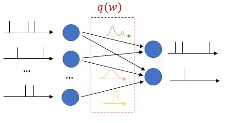
A digital twin (DT) consists of a high-fidelity virtual replica of a physical entity, the physical twin (PT), such that, in the words of DT pioneer Michael Grieves, “at its optimum, any information that could be obtained from inspecting a physical manufactured product can be obtained from its digital twin” [1]. Based on a fully automatized bi-directional flow of information [2], the DT uses the data collected from the physical world to maintain an up-to-date model of the PT, which in turn provides command and analysis functionalities to the PT (see Fig.1). With the ever-growing demand in communication resources, next-generation wireless networks will be required to adapt to a large number of scenarios, and DT platforms are increasingly seen as a promising data-driven solution to build intelligent wireless systems that can offer the necessary flexibility and responsiveness.

As depicted in Fig. 1, in a recent work to be presented at the IEEE International Conference on Communications, we consider a DT that autonomously learns a model of a wireless network, providing a safe sandbox environment for network optimization and analysis, while also enabling monitoring and prediction features. The main motivation for our work  stems from the realization that, in real-world scenarios, it is challenging to transfer sufficient data to and from the PT in a way that “any information that could be obtained from inspecting the PT can be obtained from its DT”. In light of this, we propose to leverage Bayesian methods to learn a DT model that is aware of “what it knows” as much as it is aware of “what it does not know”; taking into account the epistemic uncertainty arising from limited PT-to-DT communication [3].


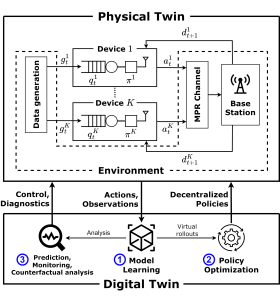
Figure 1 – The digital twin (DT) platform for the control and analysis of the communication system studied in this work. The physical twin (PT) consists of a group of K devices receiving correlated data and communicating over a shared multi-packet reception (MPR) channel. The DT platform operates along the phases of model learning (step 1) and policy optimization (step 2) ; while also enabling functionalities such as prediction, counterfactual analysis and monitoring (step 3) .


The Physical Twin

We consider a PT system made of a group of devices, referred to as agents, that attempt to communicate with a single base station (BS) over a shared multi-packet reception (MPR) channel [4]. Each agent is equipped with a limited-capacity buffer, and packet generation is taken to be correlated in-time and among agents. At any given time slot, each agent can take an action to decide whether or not to transmit a packet from their buffer, which can be received at the BS depending on the MPR channel dynamics. Upon packet reception, the BS transmits acknowledgement signals to the corresponding agents before the next time slot.

Agents cannot communicate with each other and each agent can only sense its local state, which contains information about its packet generation, buffer occupancy and BS feedback at a given time. Given the collective states and actions of all agents, the PT system evolves to a new state according to a transition distribution that is unknown to the DT and describes the packet-generation, buffer and channel dynamics.

The Digital Twin

Model Learning

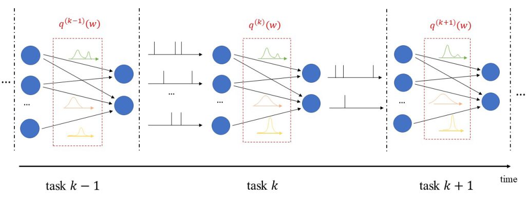
During model learning (step 1 in Fig. 1), the DT leverages sequences of states and actions collected from the PT to learn a parametric Bayesian model of the transition distribution. As opposed to frequentist learning, which only keeps the most probable model parameter, Bayesian learning keeps a (possibly infinite) ensemble of models, where the probability of each model is given by a posterior distribution. Given that all state variables are discrete, we represent the transition distribution using a categorical model and learn the corresponding posterior using the conjugate Dirichlet distribution [3]. In order to lower the spatial complexity of the model, we leverage prior information available at the DT about state transitions like data-generation clusters, known buffer dynamics, and symmetry of the MPR channel.

Policy Optimization: Safely Learn by Trial and Error

A medium access control (MAC) protocol at the PT can be established by providing each agent with a policy distribution that maps the sequence of locally observed states and actions into a new action. Using the learned model, we can safely asses new policies in virtual space by defining a reward function that yields positive values for desired behavior (e.g. successfully delivered packets) and negative penalties for undesired behavior (e.g. buffer overflow). Policy optimization (step 2 in Fig. 1) aims at providing an optimal policy to each agent that maximizes the expected sum of future rewards. This amounts to a Decentralized Markov Decision Process [5] problem that we tackle using the COunterfactual Multi-Agent (COMA) algorithm proposed in [6], in which we periodically sample a new transition distribution from the model posterior during training.

Monitoring: Let’s Agree to Disagree

After an initial model learning phase, the DT can provide monitoring features by checking whether newly received data fits previously observed transitions, or if it rather provides evidence of changed dynamics or anomalous behavior (step 3 in Fig. 1). To this end, we use a disagreement-based test metric that measures to which extent the Bayesian ensemble of models agree on the likelihood of the newly observed data. A large disagreement is taken as evidence of a large epistemic uncertainty compared to model-learning conditions, which in turn can indicate that the observation is anomalous.

Results

We evaluate the proposed DT platform on a simulated scenario consisting of 4 devices distributed across 2 data-generation clusters. The MPR channel allows for the successful delivery of one or two simultaneous packets; while more than two simultaneous transmissions cause the loss of all packets. Each device is equipped with a buffer with single-packet capacity.

During policy optimization, we reward successfully delivered packets, while we penalize buffer overflows, caused by generating a new packet on an already full buffer. We analyze the performance of the policy trained inside the Bayesian model across different sizes of model-learning datasets, and compare it to a policy trained inside the corresponding maximum a posteriori (MAP) frequentist model, and to an oracle-aided policy that is trained using the ground-truth transition distribution.


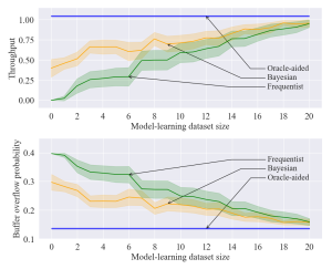
Figure 2 – Throughput and buffer overflow probability as a function of the size of the dataset available in the model learning phase for the proposed Bayesian model-based approach (orange), as well as the oracle-aided model-free (blue) and frequentist model-based (green) benchmarks.

From Fig. 2, we observe that, in regimes with high data availability during the model learning phase, both Bayesian and frequentist model-based methods yield policies with similar performance to the oracle-aided benchmark. In the low-data regime, however, Bayesian learning achieves superior performance compared to its frequentist counterpart.

To asses the performance of anomaly detection, we assume that an anomalous event occurs where a device is disconnected, resulting in an anomalous packet-generation distribution in the corresponding cluster. We compare the performance of the disagreement metric using the Bayesian model to a log-likelihood criterion using the frequentist MAP model for model-learning datasets comprising 20 and 50 transitions and report the results in the receiver operating curves (ROC) in Fig. 3.

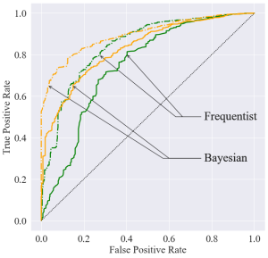
Figure 3 – Receiver operating curves (ROC) of the Bayesian (orange) and frequentist (green) anomaly detection tests for model-learning dataset sizes comprising 20 (solid lines) and 50 (dashed lines) transitions.

Bayesian anomaly detection is observed to uniformly outperform its frequentist counterpart, achieving a higher area under the ROC in Fig. 3.


For a more formal presentation of our proposed Bayesian framework for wireless networks DTs and more details on the experimental procedure, please refer to our paper at this link and to the extended version at this link.

References

[1] M. Grieves and J. Vickers, “Digital twin: Mitigating unpredictable, undesirable emergent behavior in complex systems,” in Transdisciplinary perspectives on complex systems. Springer, 2017, pp. 85–113.

[2] W. Kritzinger, M. Karner, G. Traar, J. Henjes, and W. Sihn, “Digital twin in manufacturing: A categorical literature review and classification,” IFAC-PapersOnLine, vol. 51, no. 11, pp. 1016–1022, 2018.

[3] O. Simeone, Machine Learning for Engineers. Cambridge University Press, 2022.

[4] L. Tong, Q. Zhao, and G. Mergen, “Multipacket reception in random access wireless networks: From signal processing to optimal medium access control,” IEEE Communications Magazine, vol. 39, no. 11, pp. 108–112, 2001.

[5] F. A. Oliehoek and C. Amato, A concise introduction to decentralized POMDPs. Springer, 2016.

[6] J. Foerster, G. Farquhar, T. Afouras, N. Nardelli, and S. Whiteson, “Counterfactual multi-agent policy gradients,” in Proceedings of the AAAI conference on artificial intelligence, vol. 32, no. 1, 2018.

Life-long brain-inspired learning that knows what it does not know

An emerging research topic in artificial intelligence (AI) consists in designing systems that take inspiration from biological brains. This is notably driven by the fact that, although most AI algorithms become more and more efficient (for instance, for image generation), this comes at a cost. Indeed, with architectures constantly growing in size, training a single large neural network today consumes a prohibitive amount of energy. Despite consuming only about 12W, human brains exhibit impressive capabilities, such as life-long learning.

By taking a Bayesian perspective, we demonstrate in our latest work how biologically inspired spiking neural networks (SNNs) can exhibit learning mechanisms similar to those applied in brains, which allow them to perform continual learning. As we will see, the technique also solves a key challenge in deep learning, that is, to obtain well calibrated solutions in the face of previously unseen data.


Our work

Bayesian Learning

As seen in Fig. 1, we propose to equip each synaptic weight in the SNN with a probability distribution. The distribution captures the epistemic uncertainty induced by the lack of knowledge of the true distribution of the data. This is done by assigning probabilities to model parameters that fit equally well the data, while also being consistent with prior knowledge. As a consequence, Bayesian learning is known to produce better calibrated decisions, i.e., decisions whose associated confidence better reflects the actual accuracy of the decision.

This contrasts with frequentist learning, in which the vector of synaptic weights is optimized by minimizing a training loss. The training loss is adopted as a proxy for the population loss, i.e., for the loss averaged over the true, unknown, distribution of the data. Therefore, frequentist learning disregards the inherent uncertainty caused by the availability of limited training data, which causes the training loss to be a potentially inaccurate estimate of the population loss. As a result, frequentist learning is known to potentially yield poorly calibrated, and overconfident decisions for ANNs.

Figure 1: Illustration of Bayesian learning in an SNN: In a Bayesian SNN, the synaptic weights are assigned a joint distribution, often simplified as a product distribution across weights.

We consider both real-valued (with possibly limited resolution, as dictated by deployment on neuromorphic hardware) and binary-valued synapses, parametrised by Gaussian and Bernoulli distributions, respectively. The advantages of models with binary-valued synapses, i.e., binary SNNs, include a reduced complexity for the computation of the membrane potential. Furthermore, binary SNNs are particularly well suited for implementations on chips with nanoscale components that provide discrete conductance levels for the synapses.


Continual Learning

In addition to uncertainty quantification, we apply the proposed solution to continual learning, as illustrated in Fig. 2. In continual learning, the system is sequentially presented several datasets corresponding to distinct, but related, learning tasks, where each task is selected, possibly with replacement, from a pool of tasks, and its identity is unknown to the system. Its goal is to learn to make predictions that generalize well each new task, while causing minimal loss of accuracy on previous tasks.

Figure 2: Illustration of Bayesian continual learning: the system is successively presented with similar, but different, tasks. Bayesian learning allows the model to retain information about previously learned information.

Many existing works on continual learning draw their inspiration from the mechanisms underlying the capability of biological brains to carry out life-long learning. Learning is believed to be achieved in biological systems by modulating the strength of synaptic links. In this process, a variety of mechanisms are at work to establish short-to intermediate-term and long-term memory for the acquisition of new information over time. These mechanisms operate at different time and spatial scales.


Biological Principles of Learning

One of the best understood mechanisms, long-term potentiation, contributes to the management of long-term memory through the consolidation of synaptic connections. Once established, these are rendered resistant to disruption by changing their capacity to change via metaplasticity. As a related mechanism, return to a base state is ensured after exposition to small, noisy changes by heterosynaptic plasticity, which plays a key role in ensuring the stability of neural systems. Neuromodulation operates at the scale of neural populations to respond to particular events registered by the brain. Finally, episodic replay plays a key role in the maintenance of long-term memory, by allowing biological brains to re-activate signals seen during previous active periods when inactive (i.e., sleeping).

In this work, we demonstrate how the continual learning rule we obtain exhibits some of these mechanisms. In particular, synaptic consolidation and metaplasticity for each synapse can be modeled by a precision parameter. A larger precision reduces the step size of the synaptic weight updates. During learning, the precision is increased to the degree that depends on the relevance of each synapse as measured by the estimated Fisher information matrix for the current mini-batch of examples.

Heterosynaptic plasticity, which drives the updates towards previously learned and resting states to prevent catastrophic forgetting, is obtained from first principles via an information risk minimization formulation with a Kullback-Leibler regularization term. This mechanism drives the updates of the precision and mean parameter towards the corresponding parameters of the variational posterior obtained at the previous task.

Figure 3: Predictive probabilities evaluated on the two-moons dataset after training for Bayesian learning. Top row: Real-valued synapses; Bottom row: Binary synapses.

Results

We start by considering the two-moons dataset shown in Fig. 3. Triangles indicate training points for a class “0’’, while circles indicate training points for a class “1”. The color intensity represents the predictive probabilities for frequentist learning and for Bayesian learning: the more intense the color, the higher the prediction confidence determined by the model. Bayesian learning is observed to provide better calibrated predictions, that are more uncertain outside the input regions covered by training data points. As can be seen, confidence for the Bayesian models can be mitigated by a parameter, as precised in the full text.

Figure 4: Top three classes predicted by both Bayesian and frequentist models on selected examples from the DVS-Gestures dataset. Top: real-valued synapses. Bottom: binary synapses. The correct class is indicated in bold font.

This point is further illustrated in Fig. 4 by showing the three largest probabilities assigned by the different models on selected examples from DVS-Gestures dataset, considering real-valued synapses in the top row and binary synapses in the bottom row. In the left column, we observe that, when both models predict the wrong class, Bayesian SNNs tend to do so with a lower level of certainty, and typically rank the correct class higher than their frequentist counterparts. Specifically, in the examples shown, Bayesian models with both real-valued and binary synapses rank the correct class second, while the frequentist models rank it third. Furthermore, as seen in the middle column, in a number of cases, the Bayesian models manage to predict the correct class, while the frequentist models predict a wrong class with high certainty. In the right column, we show that even when frequentist models predict the correct class and Bayesian models fail to do so, they still assign lower probabilities (i.e., <50%) to the predicted class.

Figure 5: Evolution of the average test accuracies and ECE on all tasks of the split-MNIST-DVS across training epochs, with Gaussian and Bernoulli variational posteriors, and frequentist schemes for both real-valued and binary synapses. Continuous lines: test accuracy, dotted lines: ECE, bold: current task. Blue: {0, 1}; Red: {2, 3}; Green: {4, 5}; Purple:{6, 7}; Yellow: {8, 9}.

Finally, we show results for continual learning on the MNIST-DVS dataset in Fig. 5. We show the evolution of the test accuracy and expected calibration error (ECE) on all tasks, represented with lines of different colors, during training. The performance on the current task is shown as a thicker line. We consider frequentist and Bayesian learning, with both real-valued and binary synapses. With Bayesian learning, the test accuracy on previous tasks does not decrease excessively when learning a new task, which shows the capacity of the technique to tackle catastrophic forgetting. Also, the ECE across all tasks is seen to remain more stable for Bayesian learning as compared to the frequentist benchmarks. For both real-valued and binary synapses, the final average accuracy and ECE across all tasks show the superiority of Bayesian over frequentist learning.

More details can be found in the full text at this link.

Is Accuracy Sufficient for AI in 6G? (No, Calibration is Equally Important)

AI modules are being considered as native components of future wireless communication systems that can be fine-tuned to meet the requirements of specific deployments [1]. While conventional training solutions target the accuracy as the only design criterion, the pursuit of “perfect accuracy” is generally neither a feasible nor a desirable goal. In Alan Turing’s words, “if a machine is expected to be infallible, it cannot also be intelligent”. Rather than seeking an optimized accuracy level, a well-designed AI should be able to quantify its uncertainty: It should “know when it knows”, offering high confidence for decisions that are likely to be correct, and it should “know when it does not know”, providing a low confidence level for decisions are that are unlikely to be correct. An AI module that can provide reliable measures of uncertainty is said to be well-calibrated.

Importantly, accuracy and calibration are two distinct criteria. As an example, Fig. 1 illustrates  a QPSK demodulator trained using limited number of pilots. Depending on the input, the trained probabilistic model may result in either accurate or inaccurate demodulation decisions, whose uncertainty is either correctly or incorrectly characterized.

Fig. 1. The hard decision regions of an optimal demodulator (dashed lines) and of a data-driven demodulator trained on few pilots (solid lines) are displayed in panel (a), while the corresponding probabilistic predictions for some outputs are shown in panel (b).


The property of “knowing what the AI knows/ does not know” is very useful when the AI module is used as part of a larger engineering system. In fact, well-calibrated decisions should be treated differently depending on their confidence level. Furthermore, well-calibrated models enable monitoring – by tracking the confidence of the decisions made by an AI – and other functionalities, such as anomaly detection [2].

In a recent paper from our group published on the IEEE Transaction on Signal Processing [3], we proposed a methodology to develop well-calibrated and efficient AI modules that are capable of fast adaptation. The methodology builds on Bayesian meta-learning.

To start, we summarize the main techniques under consideration.

  1. Conventional, frequentist, learning ignores epistemic uncertainty – uncertainty caused by limited data – and tends to be overconfident in the presence of limited training samples.
  2. Bayesian learning captures epistemic uncertainty by optimizing a distribution in the model parameter space, rather than finding a single deterministic value as in frequentist learning. By obtaining decisions via ensembling, Bayesian predictors can account for the “opinions” of multiple models, hence providing more reliable decisions. Note that this approach is routinely used to quantify uncertainty in established fields like weather prediction [4].
  3. Frequentist meta-learning [5], also known as learning to learn, optimizes a shared training strategy across multiple tasks, so that it can easily adapt to new tasks. This is done by transferring knowledge from different learning tasks. As a communication system example, see Fig. 2 in which the demodulator adapts quickly with only few pilots for a new frame. While frequentist meta-learning is well-suited for adaptation purpose, its decisions tend to be overconfident, hence not improving monitoring in general.
  4. Bayesian meta-learning [6,7] integrates meta-learning with Bayesian learning in order to facilitate adaptation to new tasks for Bayesian learning.
  5. Bayesian active meta-learning [8] Active meta-learning can reduce the number of meta-training tasks. By considering streaming-fashion of availability of meta-training tasks, e.g., sequential supply of new frames from which we can online meta-learn the AI modules, we were able to effectively reduce the time required for satisfiable meta-learning via active meta-learning.


Fig. 2. Through meta-learning, a learner (e.g., demodulator) can be adapted quickly using few pilots to new environment, using hyperparameter vector optimized over related learning tasks (e.g., frames with different channel conditions).


Some Results

We first show the benefits of Bayesian meta-learning for monitoring purpose by examining the reliability of its decisions in terms of calibration. In Fig. 3, reliability diagrams for frequentist and Bayesian meta-learning are compared. For an ideal calibrated predictor, the accuracy level should match the self-reported confidence (dashed line in the plots). In can be easily checked that AI modules designed by Bayesian meta-learning (right part) are more reliable than the ones with Frequentist meta-learning (left part), validating the suitability of Bayesian meta-learning for monitoring purpose. Experimental results are obtained by considering a demodulation problem.


Fig. 3. Bayesian meta-learning (right) yields reliable decisions as compared to frequentist meta-learning (left) which can be captured via reliability diagrams [9].

Fig. 4 demonstrates the impact of Bayesian active meta-learning that successfully reduces the number of required meta-training tasks. The results are obtained by considering an equalization problem.

Fig. 4. Bayesian active meta-learning actively searches for meta-training tasks that are most surprising (left), hence increasing the task efficiency as compared to Bayesian meta-learning which randomly chooses tasks to be meta-trained.


References

[1] O-RAN Alliance, “O-RAN Working Group 2 AI/ML Workflow Description and Requirements,” ORAN-WG2. AIML. v01.02.02, vol. 1, 2.

[2] C. Ruah, O. Simeone, and B. Al-Hashimi, “Digital Twin-Based Multiple Access Optimization and Monitoring via Model-Driven Bayesian Learning,” arXiv preprint arXiv:2210.05582.

[3] K.M. Cohen, S. Park, O. Simeone and S. Shamai, “Learning to Learn to Demodulate with Uncertainty Quantification via Bayesian Meta-Learning,” arXiv https://arxiv.org/abs/2108.00785

[4] T. Palmer, “The Primacy of Doubt: From Climate Change to Quantum Physics, How the Science of Uncertainty Can Help Predict and Understand Our Chaotic World,” Oxford University Press, 2022.

[5] C. Finn, P. Abbeel, and S. Levine, “Model-Agnostic Meta-Learning for Fast Adaptation of Deep Networks,” in Proceedings of the 34th International Conference on Machine Learning, vol. 70. PMLR, 06–11 Aug 2017, pp. 1126–1135.

[6] J. Yoon, T. Kim, O. Dia, S. Kim, Y. Bengio, and S. Ahn, “Bayesian Model-Agnostic Meta-Learning,” Proc. Advances in neural information processing systems (NIPS), in Montreal, Canada, vol. 31, 2018.

[7] C. Nguyen, T.-T. Do, and G. Carneiro, “Uncertainty in Model-Agnostic Meta-Learning using Variational Inference,” in Proceedings of the IEEE/CVF Winter Conference on Applications of Computer Vision, 2020, pp. 3090–3100.

[8] J. Kaddour, S. Sæmundsson et al., “Probabilistic Active Meta-Learning,” Proc. Advances in Neural Information Processing Systems (NIPS) as Virtual-only Conference, vol. 33, pp. 20 813–20 822, 2020.

[9] C. Guo, G. Pleiss, Y. Sun, and K. Q. Weinberger, “On Calibration of Modern Neural Networks,” in International Conference on Machine Learning. PMLR, 2017, pp. 1321–1330.