Motivation
Membership Inference Attacks (MIAs) pose a critical threat to machine learning models, as they enable adversaries to determine whether a particular data point was used during training. This threat becomes especially concerning in real-world settings like smart healthcare, where even a single query to a diagnostic model could reveal whether a patient’s medical record was part of the training set.

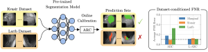
Fig. 1 Illustration of MIAs under different disclosure settings.
Depending on what the model reveals to the adversary, MIAs can take different forms. As shown in Fig. 1, in the most common setting, the attacker observes the full confidence vector (CV) output by the model for a given input. Other settings consider more restricted disclosures, such as only the true label confidence (TLC) or a decision set (DS), which contains all labels whose predicted confidence exceeds a certain threshold. Each of these disclosure modes enables different levels of privacy leakage and has motivated a range of attack strategies.
To defend against such attacks, it is essential to understand their underlying mechanisms. In other words, “know the enemy to protect oneself.” While prior work has provided valuable insights through empirical studies and theoretical analysis, several limitations remain. First, most analyses focus narrowly on TLC, overlooking other common disclosures like CV and DS. Second, existing frameworks are often tied to specific assumptions, such as differential privacy or Bayesian attackers, limiting generality. Third, prior work emphasizes tight performance bounds, rather than uncovering how key factors shape attack success. Fourth, many studies focus on high-level variables like architecture or data size, without linking them to fundamental sources of privacy leakage such as uncertainty and calibration.
We seek to understand the principled, theoretical underpinnings of why MIAs succeed in the first place through the lens of uncertainty and calibration. By formally characterizing the attacker’s advantage and linking it to intrinsic properties of the model, we provide a roadmap for privacy-aware model design that is explainable and generalizable.
Theoretical Analysis on MIAs

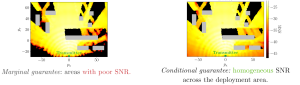
Fig.2 Illustration of LiRA-style attacks.
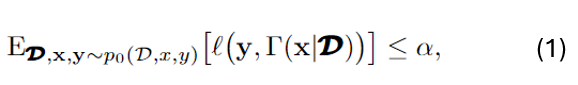
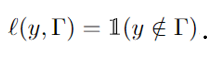
As shown in Fig. 2, we consider a class of state-of-the-art likelihood-ratio attacks (LiRA), which estimate the likelihood that a given data point was used for training by comparing the outputs of two shadow models: one trained with the target point and one without [1]-[4]. This process can be formulated as a binary hypothesis testing problem, where the attacker aims to distinguish whether the input originates from the training set (in-sample) or not (out-of-sample), based on the model’s output. The membership inference advantage, which serves as our central privacy metric, is defined as the difference between the true negative rate (TNR) and the false negative rate (FNR).
To analyze this advantage, we adopt a distributional view of the model outputs and apply information-theoretic tools. Specifically, we derive a general upper bound on the MIA advantage in Lemma 2, showing that it is controlled by the Kullback-Leibler (KL) divergence between the output distributions of the in-sample and out-of-sample shadow models. This result provides a unified way to quantify the attacker’s ability to distinguish between the two hypotheses based on distributional separation.
To interpret this bound in terms of model properties, we model the output confidence vector as a Dirichlet distribution. Within this framework, we explicitly incorporate three key factors: calibration error, aleatoric uncertainty, and epistemic uncertainty. The calibration error measures the mismatch between predicted probabilities and the true label distribution (Eq. 24). Aleatoric uncertainty captures the intrinsic randomness in the data (Eq. 23), while epistemic uncertainty reflects model uncertainty caused by limited or imperfect information available during model training (Eq. 28). Conversely, we then express the Dirichlet parameters in terms of these three factors in Eqs. (29)-(30). This formulation enables us to substitute the resulting distributions into the KL-based upper bound in Lemma 2, forming the basis for the analysis in the following.
Building on the above formulation, we further instantiate the general bound of MIA advantage under three commonly studied information disclosure settings: CV, TLC, and DS. For each case, we derive an explicit upper bound on the MIA advantage, presented in Propositions 1, 2, and 3, respectively. Each bound is expressed in terms of the three factors, enabling a detailed analysis of how these quantities influence the success of LiRA-style attacks.
Experiments

Fig.3 True advantage and bounds for the MIA advantage with CV, TLC, and DS observations as a function of relative calibration error (left), aleatoric uncertainty (middle), and epistemic uncertainty (right).
We validate our framework on CIFAR-10 with a standard convolutional neural network (CNN) and on CIFAR-100 with a ResNet classifier. Our theoretical results reveal consistent trends across all disclosure settings. As shown in Fig. 3, as the calibration error decreases, the aleatoric uncertainty increases, and the epistemic uncertainty increases, the MIA advantage becomes smaller, indicating that the model is more resistant to LiRA-style attacks. Moreover, the level of privacy risk decreases with less informative outputs, following the order CV, TLC, DS. These insights suggest practical strategies for improving privacy from the ground up, as further discussed in Appendix F.
Please refer to our paper at this link for more details.
References
[1] N. Carlini, S. Chien, M. Nasr, S. Song, A. Terzis, and F. Tramer, “Membership inference attacks from first principles,” in Proc. IEEE Symp. Secur. Privacy, May. 2022, pp. 1897–1914.
[2] H. Ali, A. Qayyum, A. Al-Fuqaha, and J. Qadir, “Membership inference attacks on DNNs using adversarial perturbations,” arXiv preprint arXiv:2307.05193, Jul. 2023.
[3] J. Ye, A. Maddi, S. K. Murakonda, V. Bindschaedler, and R. Shokri, “Enhanced membership inference attacks against machine learning models,” in Proc. ACM SIGSAC Conf. Comput. Commun. Secur., Nov. 2022, pp. 3093–3106.
[4] S. Zarifzadeh, P. Liu, and R. Shokri, “Low-cost high-power membership inference attacks,” arXiv preprint arXiv:2312.03262, Jun. 2024


Recent Comments