Motivation

Conformal risk control (CRC) [1] [2] is a recently proposed technique that applies post-hoc to a conventional point predictor to provide calibration guarantees. Generalizing conformal prediction (CP) [3], with CRC, calibration is ensured for a set predictor that is extracted from the point predictor to control a risk function such as the probability of miscoverage or the false negative rate. The original CRC requires the available data set to be split between training and validation data sets. This can be problematic when data availability is limited, resulting in inefficient set predictors. In [4], a novel CRC method is introduced that is based on cross-validation, rather than on validation as the original CRC. The proposed cross-validation CRC (CV-CRC) allows for the control of a broader range of risk functions, while proved to offer theoretical guarantees on the average risk of the set predictor, and reduced average set size with respect to CRC when the available data are limited.

Cross-Validation Conformal Risk Control

The objective of CRC is to design a set predictor with a mean risk no larger than a predefined level α, i.e.,

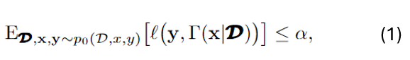
with test data input-label pair (x,y), and a set of N data pairs D.

The risk is defined between the  true label y and a predictive set Γ of labels.

VB-CRC generalizes VB-CP [2] in the sense it allows the risk taking arbitrary form under technical conditions such as boundness and monotonicity in the set. VB-CP is resorted when VB-CRC considers the special case of the miscoverage risk

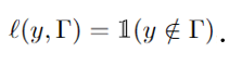
In this work, we introduce CV-CRC, which is a cross-validation-based version of VB-CRC. In a similar manner how CV-CP [5] generalizes VB-CP, CV-CRC generalizes VB-CRC. See Fig. 1 for illustration.

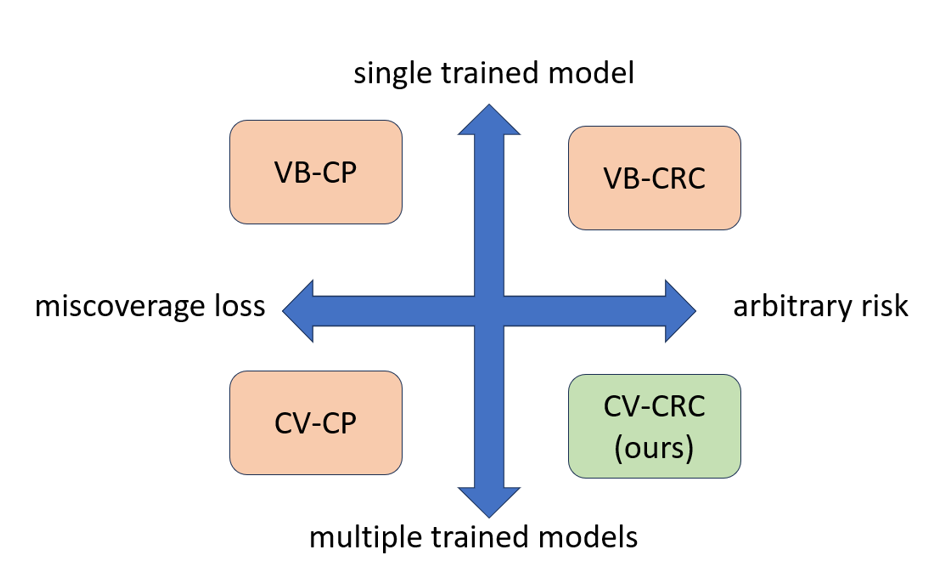
Fig. 1. (top) validation-based CRC (bottom) the proposed method, CV-CRC.

In the top panel of Fig. 2, VB-CRC is shown as the outcome of available data split into training data and validation data. The former is used to train a model, while the latter is used to post process and control a threshold λ. Upon test input x, a predictive set Γ of labels y’s is formed. In the bottom panel, CV-CRC is illustrated as a generalization. Available data is split K≤N folds, and K leave-fold-out models are trained. Then, K predictive sets are formed and merged via a threshold that is set via the trained models and the left-fold-out data.

Fig. 2. (top) validation-based CRC (bottom) the proposed method, CV-CRC.

Experiments

To illustrate the main theorem that the risk guarantee (1) is met, while the average set sizes are expected to reduce, two experiments were conducted. The first is vector regression using maximum-likelihood learning, and is shown in Fig. 3.

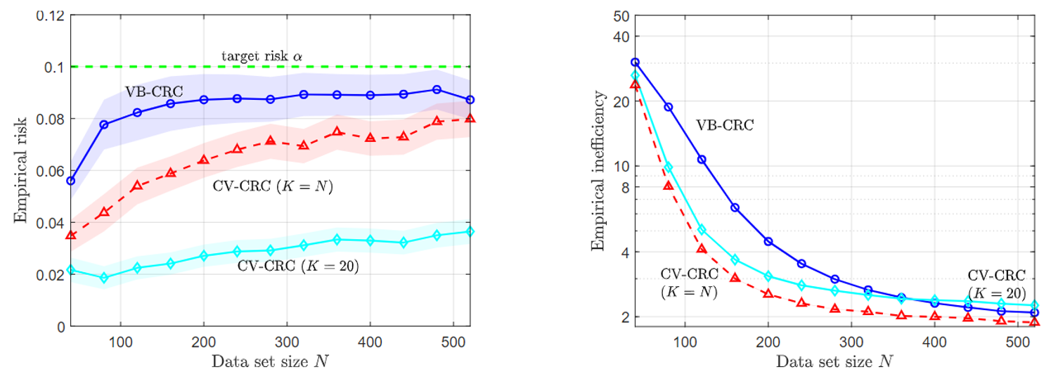
Fig. 3. VB-CRC and CV-CRC for the vector regression problem.

The second problem is a temporal point process prediction, where a point process set predictor aims to predict sets that contain future events of a temporal process with false negative rate of no more than a predefined α. As can be seen, in both problems, CV-CRC is shown to be more data-efficient in the small data regime, while holding the risk condition (1).

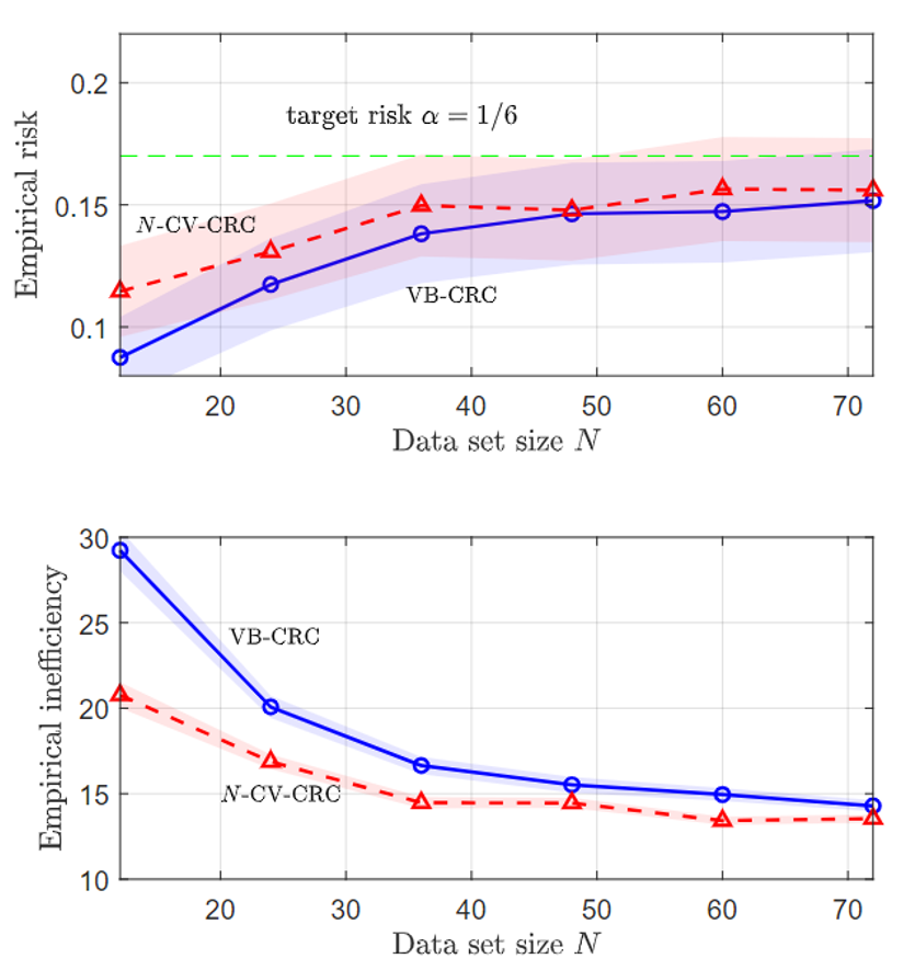
Fig. 4. VB-CRC and CV-CRC for the temporal point process prediction problem.

Full details can be found at ISIT preprint [4].

References

[1] A. N. Angelopoulos, S. Bates, A. Fisch, L. Lei, and T. Schuster, “Conformal Risk Control,” in The Twelfth International Conference on Learning Representations, 2024.

[2] S. Feldman, L. Ringel, S. Bates, and Y. Romano, “Achieving Risk Control in Online Learning Settings,” Transactions on Machine Learning Research, 2023.

[3] V. Vovk, A. Gammerman, and G. Shafer, Algorithmic Learning in a Random World. Springer, 2005, springer, New York.

[4] K. M. Cohen, S. Park, O. Simeone, and S. Shamai Shitz, “Cross-Validation Conformal Risk Control,” accepted to IEEE International Symposium on Information Theory Proceedings (ISIT2024), July 2024.

[5] R. F. Barber, E. J. Candes, A. Ramdas, and R. J. Tibshirani, “Predictive Inference with the Jackknife+,” The Annals of Statistics, vol. 49, no. 1, pp. 486–507, 2021.

Motivation

Servicing ultra-reliable and low-latency communication (URLLC) traffic typically calls for a pre-emptive allocation of resources in order to meet stringent delay constraints. A conservative static allocation of resources for URLLC may guarantee desired levels of reliability and latency, but this comes at the expense of other services, most notably enhanced mobile broadband (eMBB), which cannot use the resources reserved for URLLC. A dynamic allocation of resources, while potentially more efficient, is made challenging by the stochastic nature of URLLC data packet generation. A promising solution is the adoption of predictors of URLLC data packet generation. Concretely, with reference to Fig. 1, a base station can deploy a predictor of URLLC data packet generation for the following frame, so as to guide the adaptive allocation of slots for URLLC packets, leaving the other slots available for eMBB users.

Background

URLLC traffic

A URLLC traffic must hold two restrictions:

1. Ultra-Reliability – a portion of at least 1-α of all generated packets must be scheduled for transmission.
2. Low-Latency – Each packet should have a unique schedule resource, no later than a predefined acceptable latency.

Fig 1 (a) URLLC traffic ground true generation patterns; (b) using a predictor that underestimates the traffic dynamics leads to unreliable URLLC allocation. CP-based is able to compensate successfully; (c) using a predictor that overestimates the traffic dynamics leads to overreliable URLLC allocation, i.e., low eMBB efficiency. CP-based is able to compensate successfully this as well. 

Online Conformal Prediction

CP is a class of post-hoc calibration methods that transform standard probabilistic model into a set predictor that is guaranteed to contain the true target with probability no smaller than a predetermined coverage level [1]. Online CP alleviates the limitation of conventional CP of requiring a separate calibration data at the cost of providing time-averaged, rather than ensemble, reliability guarantees [2,3]. The adoption of CP in communication engineering was proposed in [Cohen2023ICASSP], which focused on wireless applications such as symbol demodulation, modulation classification, and received signal strength prediction.

Guaranteed Dynamic Scheduling

In our new work [4], accepted at IEEE Signal Processing Letters, we introduce a novel scheduler for URLLC packets that provides formal guarantees on reliability and latency irrespective of the quality of the URLLC traffic predictor.

Fig. 2(a) illustrates the frame-based segmentation. Fig. 2(b) shows 4 URLLC generated packets and 6 pre-emptively allocated URLLC resources, yet the latest packet is not allocated a resource within the allowed latency. In contrast, Fig. 2(c) show an allocation that meets the constraints, even though the number of URLLC resources are smaller. This leaves a better portion for eMBB traffic.

Fig. 2 (a) Frame-based timelinel; (b) miscovered allocation; (c) well-covered allocation.

The proposed method leverages recent advances in online CP, and follows the principle of dynamically adjusting the amount of allocated resources so as to meet reliability and latency requirements set by the designer. To this end, we adjust a threshold that changes between frames on the basis of a reliability condition, that controls how conservative the predictor of the next frame is.

Experiments

We consider two mismatched predictors: the first underestimates the dynamic of changes the URLLC traffic, while the second overestimates.

Fig. 3 investigates of the impact of such mismatches between URLLC model parameter and ground-truth model parameter. For some parameters values of mismatch, the conventional scheduler does not hold reliability to the desired level, while for the other it may result in over reliability. The conventional scheduler is significantly affected by a mismatch between predictor and ground-truth packet generation mechanism, yielding either ill empirical coverage (below 1-α) or over coverage. In contrast, the CP-based predictor is able to flatten the coverage to asymptotically reach the long-term target 1-α.

.

Fig. 3 Empirical URLLC reliability rate and eMBB efficiency. CP-based scheduler flattens out the coverage

Full details can be found at this SPL preprint [4].

[1] Vovk, Vladimir, Alexander Gammerman, and Glenn Shafer. “Algorithmic learning in a random world,” Vol. 29. New York: Springer, 2005.

[2] Gibbs, Isaac, and Emmanuel Candes. “Adaptive conformal inference under distribution shift.” Advances in Neural Information Processing Systems 34 (2021): 1660-1672.

[3] Feldman, Shai, Stephen Bates, and Yaniv Romano. “Conformalized Online Learning: Online Calibration Without a Holdout Set.” arXiv preprint arXiv:2205.09095 (2022).

[4] Cohen, Kfir M., Sangwoo Park, Osvaldo Simeone, Petar Popovski, and Shlomo Shamai. “Guaranteed Dynamic Scheduling of Ultra-Reliable Low-Latency Traffic via Conformal Prediction.” To appear in Signal Processing Letters, [online] arXiv preprint arXiv:2302.07675 (2023).

Motivation

Artificial intelligence (AI) models typically report a confidence measure associated with each prediction, which reflects the model’s self evaluation of the accuracy of a decision. Notably, neural networks implement probabilistic predictors that produce a probability distribution across all possible values of the output variable. As an example, Fig. 1 illustrates the operation of a neural network-based demodulator, which outputs a probability distribution on the constellation points given the corresponding received baseband sample. The self-reported model confidence, however, may not be a reliable measure of the true, unknown, accuracy of the prediction, in which case we say that the AI model is poorly calibrated. Poor calibration may be a substantial problem when AI-based decisions are processed within a larger system such as a communication network.

Fig. 1 Accuracy and calibration are different properties of probabilistic predictiors.

Set Predictors

A set predictor is defined as a set-valued function that maps an input to a subset of the output domain based on a data set. As illustrated in the example of Fig. 1, it depends in general on an input, and can be taken as a measure of the uncertainty of the predictor. The performance of a set predictor is evaluated in terms of coverage and inefficiency. Coverage refers to the probability that the true label is included in the predicted set; while inefficiency refers to the average size of the predicted set. There is a clear a trade-off between two metrics.

Given a probabilistic predictor, one can construct a set predictor by relying on the confidence levels reported by the model. To this end, one can construct the smallest subset of the output domain that covers a fraction 1 − α of the probability designed by the trained model given an input. For poorly calibrated predictors, this approach cannot satisfy the coverage condition for the given desired miscoverage level α.

Conformal Prediction

In our new work [3], presented at ICASSP2023, we applied three different conformal prediction schemes for a demodulation problem:

1. Validation-based (VB) [1] – which partitions the available data set into training and validation sets. Uses the first set to train a model, and the second for calibration purpose.
2. Cross-Validation-based (CV) [2] – which trains multiple models, each using all the available data set excluding one data point, that acts as a validation example. While increasing computational complexity, in general it reduces the inefficiency of the predictive sets.
3. K-fold CV-based (K-CV) [2] – which cross-validates using a fold rather than a single point. K different models are trained using a leave-fold-out approach. This is a generalization of CV-CP set predictors that strike a balance between complexity and inefficiency by reducing the total number of model training phases to K.

Experiments

Fig. 2 shows the empirical coverage level and Fig. 3 shows the empirical inefficiency as a function of the size N of the available data set D. From Fig. 2, we first observe that the naïve set predictor, with both frequentist and Bayesian learning, does not meet the desired coverage level in the regime of a small number N of available samples. In contrast, all CP methods provide coverage guarantees, achieving coverage rates at least 1 − α. From Fig. 3, we observe that the size of the predicted sets, and hence the inefficiency, decreases as the data set size increases. Furthermore, due to their efficient use of the available data, CV and K-CV predictors have a lower inefficiency as compared to VB predictors. Finally, Bayesian NC scores are generally seen to yield set predictors with lower inefficiency, confirming the merits of Bayesian learning in terms of calibration.

Overall, the experiments confirm that all the CP-based predictors are all well-calibrated with small average set prediction size, unlike naïve set predictors that built directly on the self-reported confidence levels of conventional probabilistic predictors.

Fig. 2 Empirical coverage as function of data set size

Fig. 3 Empirical inefficiency as function of data set size

Please see preprint of the ICASSP23 paper for full details.

[1] Vovk, Vladimir, Alexander Gammerman, and Glenn Shafer. “Algorithmic learning in a random world,” Vol. 29. New York: Springer, 2005.

[2] Barber, Rina Foygel, Emmanuel J. Candes, Aaditya Ramdas, and Ryan J. Tibshirani. “Predictive inference with the jackknife+.” (2021): 486-507.

[3] Cohen, Kfir M., Park, Sangwoo,  Simeone, Osvlado, and Shamai, Shlomo (Shitz). “Calibrating AI Models for Wireless Communications via Conformal Prediction,” to appear in ICASSP 2023 [Online]. Available: https://arxiv.org/abs/2212.07775