Problem
Training state-of-the-art Artificial Neural Network (ANN) models requires distributed computing on large mixed CPU-GPU clusters, typically over many days or weeks, at the expense of massive memory, time, and energy resources, and potentially of privacy violations. Alternative solutions for low-power machine learning on resource-constrained devices have been recently the focus of intense research. In our recently accepted paper at ICASSP 2020, we study the convergence of two such recent lines of inquiries.
On the one hand, Spiking Neural Networks (SNNs) are biologically inspired neural networks in which neurons are dynamic elements processing and communicating via sparse spiking signals over time, rather than via real numbers, enabling the native processing of time-encoded data, e.g., from DVS cameras. They can be implemented on dedicated hardware, offering energy consumptions as low as a few picojoules per spike. A more thorough introduction to probabilistic SNNs can be found in this previous blog post.
On the other hand, Federated Learning (FL) allows devices to carry out collaborative learning without exchanging local data. This makes it possible to train more effective machine learning models by benefiting from data at multiple devices with limited privacy concerns. FL requires devices to periodically exchange information about their local model parameters through a parameter server. It has become de-facto standard for training ANNs over large numbers of distributed devices.
System model
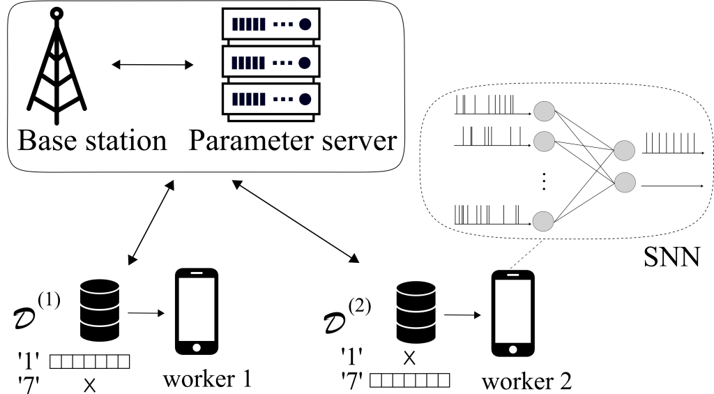
Figure 1 Federated Learning (FL) model under study: Mobile devices collaboratively train on-device SNNs based on different, heterogeneous, and generally unbalanced local data sets, by communicating through a base station (BS).
In our work, as seen in Figure 1, we consider a distributed edge computing architecture in which N mobile devices communicate through a Base Station (BS) in order to perform the collaborative training of local SNN models via FL. Each device holds a different local data set. The goal of FL is to train a common SNN-based model without direct exchange of the data from the local data sets.
FL proceeds in an iterative fashion across T global time-steps. To elaborate, at each global time-step, the devices refine their local model, based on their local datasets. Every τ iterations, they will also transmit their updated local model parameters to the BS, which will in turn compute a centralized averaged parameter and send it back to the devices. This global averaged parameter will be used at the beginning of the next iteration.
An SNN is a network of spiking neurons connected via an arbitrary directed graph, possibly with cycles (see Figure 2). SNNs process information through time, based on a local clock. At each local algorithmic time-step, each neuron receives the signals emitted by the subset of neurons connected to it through directed links, known as synapses. Neurons in the network will then output a binary signal, either ‘0’ or ‘1’. The instantaneous spiking probability of a neuron is determined by its past spiking behaviour and the previous spikes of its pre-synaptic neurons. SNNs are trained over sequences of S local algorithmic time-steps, made of D examples of length S’. In an image classification task, an example could be an image encoded as a binary signal.
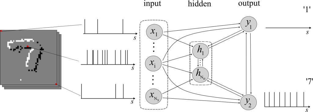
Figure 2 Example of an internal architecture for an on-device SNN.
In FL-SNN, we cooperatively train distributed on-device SNNs thanks to Federated Learning. To that end, we derived a novel algorithm, for which the time scales involved are summarized in Figure 3. Each global algorithmic iteration t corresponds to Δs local SNN time-steps, and the total number S of SNN local algorithmic time steps and the number T of global algorithmic time steps during the training procedure are hence related as S = DS’ = T∆s.
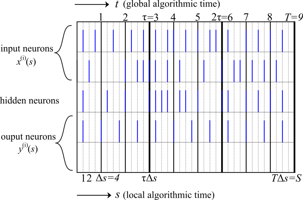
Figure 3 Illustration of the time scales involved in the cooperative training of SNNs via FL for τ = 3 and ∆s = 4.
Experiments
We consider a classification task based on the MNIST-DVS dataset. The training dataset is composed of 900 examples per class and the test dataset is composed of 100 samples per class. We consider 2 devices which have access to disjoint subsets of the training dataset. In order to validate the advantages of FL, we assume that the first device has only samples from class ‘1’ and the second only from class ‘7’. We train over D = 400 randomly selected examples from the local data sets, which results in S = DS’ = 32,000 local time-steps.
As a baseline, we consider the test loss at convergence for the separate training of the two SNNs. In Figure 4, we plot the local test loss normalized by the mentioned baseline as a function of the global algorithmic time. A larger communication period τ is seen to impair the learning capabilities of the SNNs, yielding a larger final value of the loss. In fact, for τ = 400, after a number of local iterations without communication, the individual devices are not able to make use of their data to improve performance.
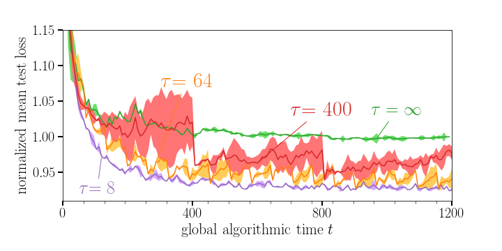
Figure 4 Evolution of the mean test loss during training for different values of the communication period τ. Shaded areas represent standard deviations over 3 trials
One of the major flaws of FL is the communication load incurred by the need to regularly transmit large model parameters. To partially explore this aspect, in the paper, we consider exchanging only a subset of synaptic weights during global iterations. We refer to the text at this link for details.
Recent Comments