Author: Sharu Jose

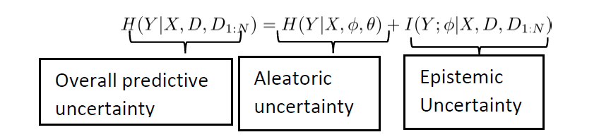
The overall predictive uncertainty of a trained predictor comprises of two main contributions: the aleatoric uncertainty arising due to inherent randomness in the data generation process and the epistemic uncertainty resulting due to limitations of available training data. While the epistemic uncertainty, also called minimum excess risk, can be made to vanish with increasing training data, the aleatoric uncertainty is independent of the data. In our recent work accepted to AISTATS 2022, we provide an information-theoretic quantification of the epistemic uncertainty arising in the broad framework of Bayesian meta-learning.

Problem Formulation

In conventional Bayesian learning, the model parameter   that describes the data generating distribution is assumed to be random and is endowed with a prior distribution. This distribution is conventionally chosen based on prior knowledge about the problem. In contrast,  Bayesian meta-learning (see Fig. 1 below) aims to automatically infer this prior distribution by observing data from several related tasks. The statistical relationship among the tasks is accounted for via a global latent hyperparameter .  Specifically, the model parameter for each observed task  is drawn according to a shared prior distribution   with shared global hyperparameter . Following the Bayesian formalism, the hyperparameter is assumed to be random and distributed according to a hyper-prior distribution .

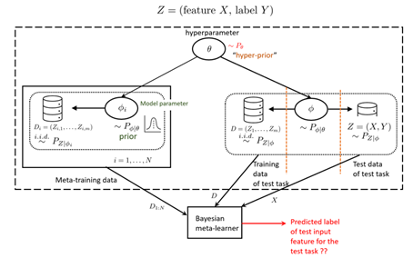
Figure 1: Bayesian meta-learning decision problem

The data from the observed related tasks, collectively called meta-training data, is used to reduce the expected loss incurred on a test task. The test task is modelled as generated by an independent model parameter  with the same shared hyperparameter. This model parameter underlies the generation of a test task training data, used to infer the task-specific model parameter, as well as a test data sample from the test task. The Bayesian meta-learning decision problem is to predict the label corresponding to test input feature of the test task, after observing the meta-training data and the training data of the test task.

A meta-learning decision rule    thus maps the meta-training data, the test task training data and test input feature to an action space.  The Bayesian meta-risk can be defined as the minimum expected loss incurred over all meta-learning decision rules, i.e., .  In the genie-aided case when the model parameter and hyper-parameter are known, the genie-aided Bayesian risk is defined as  . The epistemic uncertainty, or minimum excess risk, corresponds to the difference between the Bayesian meta-risk and Genie-aided meta-risk as  .

Main Result

Our main result shows that under the log-loss, the minimum excess meta-risk can be exactly characterized using the conditional mutual information

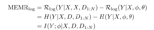
where H(A|B)  denotes the conditional entropy of A given B and  I(A;B|C) denotes the conditional mutual information between A and B given C.  This in turn implies that

More importantly, we show that the epistemic uncertainty is contributed by two levels of uncertainties – model parameter level and hyperparameter level as

which scales in the order of 1/Nm+1/m, and vanishes as both the number of observed tasks and per-task data samples go to infinity. The behavior of the bounds is illustrated for the problem of meta-learning the Bayesian neural network prior for regression tasks in the figure below.

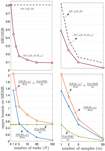
Figure 2: Performance of MEMR and derived upper bounds as a function of number of tasks and per-task data samples

Problem

Conventional learning optimizes model parameters using a training algorithm, while meta-learning optimizes the hyperparameters of a training algorithm. A meta-learner has access to data from a class of tasks, and its goal is to ensure that the resulting training algorithm, also called base-learner, performs well on any new tasks from the same class. For example, the base-learner could be a stochastic gradient descent (SGD) algorithm with hyperparameters like initialization or learning rate.

The tasks observed during meta-training are conventionally assumed to belong to a task environment, which defines a distribution over the class of tasks, where each task has an associated data distribution. The statistical properties of the task environment then determine the similarity between the tasks. Intuitively, if the average “distance” between data distributions of any two tasks in the task environment is small, the meta-learner should be able to learn a suitable shared hyperparameter by observing fewer number of tasks.

In our recent work accepted to ISIT 2021, we build on the above observation and address the following questions for a fixed base-learner and meta-learner: How to measure task similarity? Given the level of similarity of the tasks in the environment, how many tasks and how much data per task should be observed to guarantee that the target average population loss for new tasks can be well approximated using the available meta-training data?

The difference between the average population loss on a new, previously unseen, meta-test task and the meta-training loss on the data gathered from the meta-training tasks is the meta-generalization gap, and is a measure of the generalization capability of the meta-learner. Our main contribution is a novel information theoretic bound on the average absolute value of the meta-generalization gap, that explicitly captures the impact of task relatedness, the number of tasks, and the number of data samples per task on meta-generalization.

Results

 Although information-theoretic bounds on generalization performance of meta-learning have been previously studied – in both average and high probability PAC-Bayesian settings, they fail to capture the impact of task similarity in meta-generalization gap.  We identify the following distinguishing components of our analysis that enable the explicit characterization of task similarity:

• Performance metric – Earlier work on meta-learning considers the absolute average meta-generalization gap (  ) as the performance metric, that computes the absolute value of the average of the meta-generalization gap over selection of meta-training and meta-test tasks. By “mixing up’’ the tasks via first averaging over the tasks and then taking the absolute value, the metric fails to account for the dissimilarity between the training and test tasks.
  • We mitigate this drawback via a new metric, namely the average absolute value of the meta-generalization gap ( ). This metric first computes the absolute value of meta-generalization gap for a  given selection of meta-test task and meta-training tasks, and then  average it over all such selections. By doing so, this metric distinguishes the contribution of each selection of meta-training   and  meta-test tasks, and thus capture the role of similarity between tasks, in the generalization performance of a meta-learner. Moreover, in contrast to absolute average meta-generalization gap, this new metric is non-vanishing in the asymptotic limit of large number of tasks and per-task training samples. This clearly reflects that the meta-training loss cannot provide an asymptotically accurate  estimate of meta-test loss, which is evaluated on a priori unknown task.

• Measures of Task Relatedness – A task environment is said to be  epsilon- related if the average “distance” between the data distributions of any two tasks in the environment is upper bounded by epsilon.  We consider KL divergence based as well as the Jensen-Shannon based distance measures. While the former can be unbounded, the latter is always bounded.

Using the above defined measures of performance and task relatedness, we obtain novel information theoretic bounds on the average absolute value of the meta-generalization gap. The obtained bound demonstrates that (a) as the task dissimilarity parameter  increases, more number of meta-training tasks are required to ensure meta-generalization, and that  (b) there exists a non-vanishing gap, which arises due to task dissimilarity, even in the limit of large number of meta-training tasks and meta-test tasks.

We also study examples where the obtained bound can be evaluated analytically or numerically. For the example of ridge regression with meta-learned bias, we illustrate the impact of task dissimilarity parameter on the two performance metrics, and their corresponding upper bounds,  in the following figure. As can be seen, while the absolute average meta-generalization gap metric appears to be largely insensitive to task dissimilarity, our metric reveals the role of task similarity, as captured by the bounds derived in the paper.