Category: Uncategorized (Page 2 of 2)

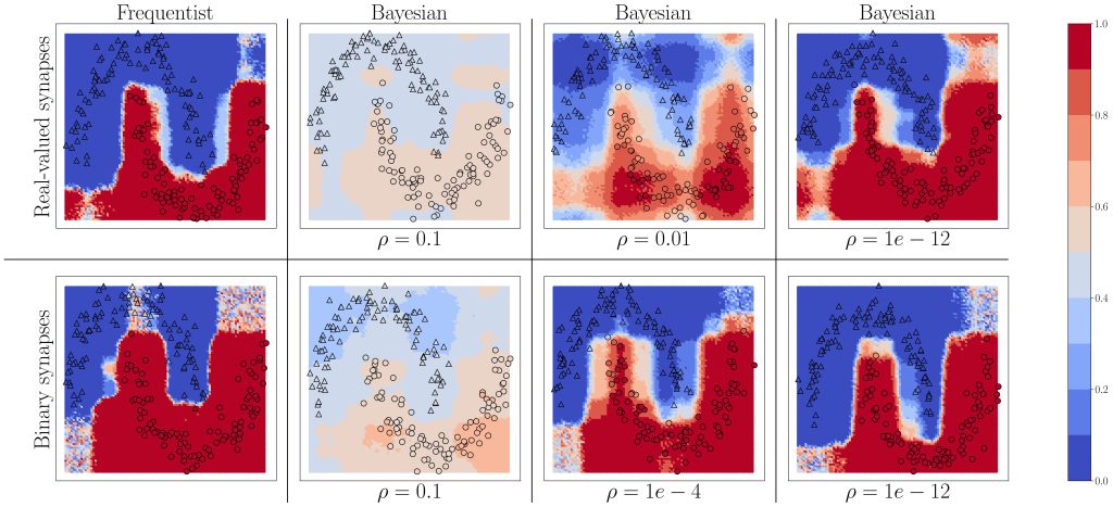
Whilst the true impact of quantum computers is anybody’s guess, there seems to be some consensus on the advantages offered by near-term devices in modeling more complex probability distributions. These distributions can be used to model complex particle interactions, e.g., in quantum chemistry, or, as we will see next, to train principled machine learning models – in this case, binary Bayesian neural networks – and enable fast adaptation to new learning tasks from few training examples.

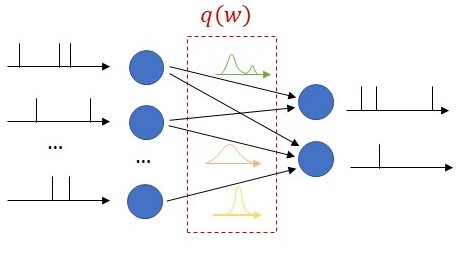
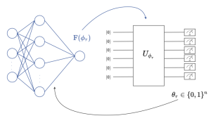
Fig. 1. (left) A binary Bayesian neural network, i.e., a neural network with stochastic binary weights, is trained to carry out a learning task. (right) The probability distribution of the binary weights of the neural network is modelled by a Born machine, i.e., by a parametric quantum circuit (PQC), leveraging the PQC’s capacity to model complex distributions [1].

Setting

In our latest work, accepted for presentation at the IEEE MLSP, we are interested in training Bayesian binary neural networks, i.e., classical neural networks with stochastic binary weights, in a sample-efficient manner by means of meta-learning, as illustrated in Fig. 1. The key idea of this work is to model the distribution of the binary weights via a Born machine, i.e., via a probabilistic parametric quantum circuit (PQC), due to the capacity of PQCs to efficiently implement complex probability distributions [1]-[4]. We propose a novel method that integrates meta-learning with the gradient-based optimization of quantum Born machines [3], with the aim of speeding up adaptation to new learning tasks from few examples.

Born Machines

A Born machine produces random binary strings  , where    denotes the total number of model parameters, by measuring the output of a PQC  defined by parameters  .

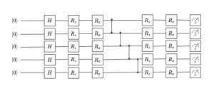
Fig. 2. Hardware-efficient ansatz for a Born machine. All qubits are initialized in the ground state. The rotations are parametrized by the entries of the variational vector.

As illustrated in Fig. 2, the PQC takes the initial state    of n qubits as an input, and operates on it via a sequence of unitary gates described by a unitary matrix   . This operation outputs the final quantum state

which is measured in the computational basis to produce a random binary string . Note that each basis vector of the computational basis corresponds to one of all the possible 2^n patterns of model parameters  .

The PQC can be implemented using a hardware-efficient ansatz [2], in which a layer of one-qubit unitary gates, parametrized by vector , is followed by a layer of fixed, entangling, two-qubit gates. This pattern can be repeated any number of times, building a progressively deeper circuit. Another option is using the mean-field ansatz that does not use entangling gates, and only relies on one-qubit gates.

By Born’s rule (hence the name of the circuit), the probability distribution of the output model parameter vector is given by

Importantly, Born machines only provide samples, while the actual distribution above can only be estimated by averaging multiple measurements of the PQC’s outputs. Therefore, Born machines model implicit distributions, and only define a stochastic procedure that directly generates samples.

Some Results

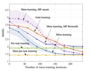
Fig. 3 illustrate the results in terms of the prediction root mean squared error (RMSE) as a function of the number of meta-training iterations. By comparison with conventional per-task learning, the figure illustrates the capacity of both joint learning and meta-learning to transfer knowledge from the meta-training to the meta-test task, with hardware-efficient (HE) and mean-field (MF) quantum meta-learning clearly outperforming joint learning. For example, HE meta-learning requires around 150 meta-training iterations to achieve the same RMSE ideal per-task training, whilst joint-learning requires more than 200 to achieve comparable performance. The HE ansatz performs best, due to the use of entangling unitaries; however, the MF ansatz approaches the minimal RMSE after 230 iterations. The classical solution based on MF Bernoulli does not achieve lower RMSE than the quantum-aided meta-learning schemes, even with joint learning.

Fig. 3. Average RMSE for a new, meta-test, task as a function of the number of meta-training iterations. The results are averaged over 5 independent trials.

Please see the paper for a more detailed exposition, available here.

References

[1] Arute, F., Arya, K., Babbush, R., Bacon, D., Bardin, J.C., Barends, R., Biswas, R., Boixo, S., Brandao, F.G., Buell, D.A., et al.: Quantum supremacy using a programmable superconducting processor. Nature 574(7779), 505–510 (2019)
[2] Kandala, A., Mezzacapo, A., Temme, K., Takita, M., Brink, M., Chow, J.M., Gambetta, J.M.: Hardware-efficient variational quantum eigensolver for small molecules and quantum magnets. Nature 549(7671), 242–246 (2017)
[3] Liu, J.G., Wang, L.: Differentiable learning of quantum circuit Born machines. Physical Review A 98(6), 062324 (2018)
[4] Sweke, R., Seifert, J.P., Hangleiter, D., Eisert, J.: On the quantum versus classical learnability of discrete distributions. Quantum 5, 417 (2021)

In 1959 Richard Feynman gave an after-dinner talk at an American Physics Society meeting in Pasadena entitled “There’s Plenty of Room at the Bottom”,  crediting Edward Fredkin for inspiration.  In his talk, the transcription of which would later become a landmark paper in quantum computation and simulation [1], he takes some existing ideas — computation is a physical process, perhaps even a quantum mechanical one — and makes a particularly famous statement:

”I’m not happy with all the analyses that go with just classical theory, because Nature isn’t classical, dammit, and if you want to make a simulation of Nature, you’d better make it quantum mechanical, and by golly it’s a wonderful problem!”

But how can we simulate the quantum mechanical nature of Nature? This new kind of machine would become the quantum computer, and from then on, quantum computing has been on a journey with many ups and downs. Nowadays, excitement seems to be in the air again as quantum machine learning, a hybrid research discipline that combines machine learning and quantum computing, has emerged as a potential practical use of quantum hardware. Generally, quantum machine learning methods apply classical optimization routines to select parameters that define the operation of a quantum circuit. Alternative approaches, which may be more promising in the short term, involve hybrid quantum-classical models, where classical computation, e.g., for feature extraction, is combined with quantum parametric circuits [2].

Our Work

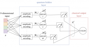
In our latest work, published in the IEEE Signal Processing Letters, we focus on the hybrid classical-quantum two-layer architecture illustrated in Fig. 1.

Fig. 1. In the studied hybrid classical-quantum classifier, a quantum hidden layer, fed via amplitude encoding and consisting of quantum generalized linear models (QGLMs), is followed by a classical combining output layer with a single classical GLM (CGLM) neuron. All weights and activations are binary.

In it, a first layer of quantum generalized linear models (QGLMs) is followed by a second classical combining layer. The input to the first, hidden, layer is obtained via amplitude encoding (see, e.g., [3]). Several implementations of QGLM neurons have been proposed in the literature using different quantum circuits. Given a binary input sample  and an N-dimensional vector of binary weights, the main goal of these circuits is to produce a stochastic binary output with probabilities which are a function of the inner product

between the input state and the amplitude-encoded binary weight vector

Different solutions, along with the resulting QGLM neuron’s response functions are given in the paper. For this hybrid model, we introduced a stochastic variational optimization (SVO) approach [4] that enables the joint training of quantum and classical layers via stochastic gradient descent. The proposed SVO-based training strategy operates in a relaxed continuous space of variational classical parameters.

Some Results

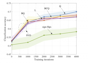
We show the classification accuracy, which is defined as the ratio of the number of accurate predictions over the total number of predictions made by the model, in Fig. 2 as a function of the training iterations.

Fig. 2. Classification accuracy as a function of the training iteration for the benchmark sign-flips scheme [5] and the proposed SVO-based procedure for the BAS data set. The results are averaged over 5 independent trials.

The proposed SVO scheme is seen to achieve high classification accuracy for all of the considered response functions. In particular, the QGLM using the Quadratic (Q) response function yields fastest convergence and achieves the best performance. Due to the additional bias terms resulting from the swap test routine, the QGLMs relying on the Biased quadratic (BQ) and Biased centered quadratic (BCQ) response functions are slower to learn, but ultimately converge after around 3000 training iterations.

Please see the paper for a more extensive presentation, available here

Code, alongside a tutorial, are available here

References

[1] R. P. Feynman et al., “Simulating physics with computers,” Int. j. Theor. phys, vol. 21, no. 6/7, 1982.
[2] A. Mari, T. R. Bromley, J. Izaac, M. Schuld, and N. Killoran, “Transfer learning in hybrid classical-quantum neural networks,” Quantum, vol. 4, p. 340, 2020.
[3] M. Schuld and F. Petruccione, Machine Learning with Quantum Computers. Springer, 2021.
[4] T. Bird, J. Kunze, and D. Barber, “Stochastic variational optimization,” arXiv preprint arXiv:1809.04855, 2018.
[5] F. Tacchino, C. Macchiavello, D. Gerace, and D. Bajoni, “An artificial neuron implemented on an actual quantum processor,” npj Quantum Information, vol. 5, no. 1, pp. 1–8, 2019

The overall predictive uncertainty of a trained predictor comprises of two main contributions: the aleatoric uncertainty arising due to inherent randomness in the data generation process and the epistemic uncertainty resulting due to limitations of available training data. While the epistemic uncertainty, also called minimum excess risk, can be made to vanish with increasing training data, the aleatoric uncertainty is independent of the data. In our recent work accepted to AISTATS 2022, we provide an information-theoretic quantification of the epistemic uncertainty arising in the broad framework of Bayesian meta-learning.

Problem Formulation

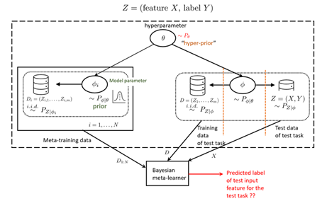
In conventional Bayesian learning, the model parameter   that describes the data generating distribution is assumed to be random and is endowed with a prior distribution. This distribution is conventionally chosen based on prior knowledge about the problem. In contrast,  Bayesian meta-learning (see Fig. 1 below) aims to automatically infer this prior distribution by observing data from several related tasks. The statistical relationship among the tasks is accounted for via a global latent hyperparameter .  Specifically, the model parameter for each observed task  is drawn according to a shared prior distribution   with shared global hyperparameter . Following the Bayesian formalism, the hyperparameter is assumed to be random and distributed according to a hyper-prior distribution .

Figure 1: Bayesian meta-learning decision problem

The data from the observed related tasks, collectively called meta-training data, is used to reduce the expected loss incurred on a test task. The test task is modelled as generated by an independent model parameter  with the same shared hyperparameter. This model parameter underlies the generation of a test task training data, used to infer the task-specific model parameter, as well as a test data sample from the test task. The Bayesian meta-learning decision problem is to predict the label corresponding to test input feature of the test task, after observing the meta-training data and the training data of the test task.

A meta-learning decision rule    thus maps the meta-training data, the test task training data and test input feature to an action space.  The Bayesian meta-risk can be defined as the minimum expected loss incurred over all meta-learning decision rules, i.e., .  In the genie-aided case when the model parameter and hyper-parameter are known, the genie-aided Bayesian risk is defined as  . The epistemic uncertainty, or minimum excess risk, corresponds to the difference between the Bayesian meta-risk and Genie-aided meta-risk as  .

Main Result

Our main result shows that under the log-loss, the minimum excess meta-risk can be exactly characterized using the conditional mutual information

where H(A|B)  denotes the conditional entropy of A given B and  I(A;B|C) denotes the conditional mutual information between A and B given C.  This in turn implies that

More importantly, we show that the epistemic uncertainty is contributed by two levels of uncertainties – model parameter level and hyperparameter level as

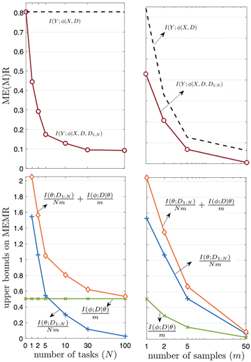
which scales in the order of 1/Nm+1/m, and vanishes as both the number of observed tasks and per-task data samples go to infinity. The behavior of the bounds is illustrated for the problem of meta-learning the Bayesian neural network prior for regression tasks in the figure below.

Figure 2: Performance of MEMR and derived upper bounds as a function of number of tasks and per-task data samples

Problem

An essential property of any wireless channel is the fact that it is a shared medium, much like the air through which sound propagates is shared among the participants of a conversation. As a result, communication engineers must deal with the resulting interference,  which may substantially limit the reliability and the achievable rates in a wireless communication system. A proven remedy is to adapt the transmission power to current channel conditions, which was successfully addressed by the data-driven methodology introduced in [1] in which the power control policy is parametrized by a random edge graph neural network (REGNN).

In our recent work to be presented at SPAWC 2021, we focus on the higher-level problem of facilitating adaptation of the power control policy. We consider the case where the topology of the network varies across periods of operation of the system, with each period being in turn characterized by time-varying channel conditions. In order to facilitate fast adaptation of the power control policy — in terms of data and iteration requirements — we integrate meta-learning with REGNN training.

Meta-learning Solution

Our meta-learning solution leverages channel state information (CSI) data from a number of previous periods to optimize an adaptation procedure that facilitates fast adaptation on a new topology to be encountered in a future period. We specifically adopt first-order meta-learning methods, namely first-order model agnostic meta-learning (FOMAML) [2] and REPTILE [3] that parametrize the adaptation procedure via its initialization within each period. While GNNs are known to be robust to changes in the topology, the proposed integration of meta-learning and REGNNs is shown to offer significant improvements in terms of sample and iteration efficiency.

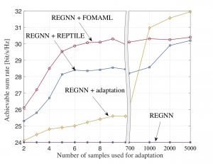
Fig 1. Sum rate as a function of the number of samples used for adaptation, for a network with dynamic size.

Some Results

The achievable sum rate with respect to the number of CSI samples used for adaptation is illustrated in Fig. 1 for a network in which the number of transmitters and receivers changes in each period. Meta-learning, via both FOMAML and REPTILE, is seen to adapt quickly to the new topology, outperforming conventional REGNN, even when allowing for fine-tuning of the later. This significant improvement can be attributed to the variability of the topologies observed across periods in the considered scenario, which makes the joint training approach in [1] ineffective. That said, when the number of samples for adaptation is sufficiently large, conventional REGNN training as in [1] outperforms meta-learning, as the initialization obtained by meta-learning induces a more substantial bias than joint training due to the mismatch in the conditions assumed for the updates on meta-training and meta-testing tasks (i.e., the different number of samples used for meta-training and adaptation).

Please see the paper for more results and a more extensive analysis, which is available here

[1] M. Eisen and A. Ribeiro, “Optimal wireless resource allocation with random edge graph neural networks,”IEEE Transactionson Signal Processing, vol. 68, pp. 2977–2991, April, 2020.

[2] C. Finn, P. Abbeel, and S. Levine, “Model-agnostic meta-learning for fast adaptation of deep networks,” inProc. InternationalConference on Machine Learning (PMLR). Sydney, 6–11 August, 2017, pp. 1126–1135.

[3] A. Nichol, J. Achiam, and J. Schulman, “On first-order meta-learning algorithms,”arXiv preprint arXiv:1803.02999, 2018.

Problem

Conventional learning optimizes model parameters using a training algorithm, while meta-learning optimizes the hyperparameters of a training algorithm. A meta-learner has access to data from a class of tasks, and its goal is to ensure that the resulting training algorithm, also called base-learner, performs well on any new tasks from the same class. For example, the base-learner could be a stochastic gradient descent (SGD) algorithm with hyperparameters like initialization or learning rate.

The tasks observed during meta-training are conventionally assumed to belong to a task environment, which defines a distribution over the class of tasks, where each task has an associated data distribution. The statistical properties of the task environment then determine the similarity between the tasks. Intuitively, if the average “distance” between data distributions of any two tasks in the task environment is small, the meta-learner should be able to learn a suitable shared hyperparameter by observing fewer number of tasks.

In our recent work accepted to ISIT 2021, we build on the above observation and address the following questions for a fixed base-learner and meta-learner: How to measure task similarity? Given the level of similarity of the tasks in the environment, how many tasks and how much data per task should be observed to guarantee that the target average population loss for new tasks can be well approximated using the available meta-training data?

The difference between the average population loss on a new, previously unseen, meta-test task and the meta-training loss on the data gathered from the meta-training tasks is the meta-generalization gap, and is a measure of the generalization capability of the meta-learner. Our main contribution is a novel information theoretic bound on the average absolute value of the meta-generalization gap, that explicitly captures the impact of task relatedness, the number of tasks, and the number of data samples per task on meta-generalization.

Results

 Although information-theoretic bounds on generalization performance of meta-learning have been previously studied – in both average and high probability PAC-Bayesian settings, they fail to capture the impact of task similarity in meta-generalization gap.  We identify the following distinguishing components of our analysis that enable the explicit characterization of task similarity:

• Performance metric – Earlier work on meta-learning considers the absolute average meta-generalization gap (  ) as the performance metric, that computes the absolute value of the average of the meta-generalization gap over selection of meta-training and meta-test tasks. By “mixing up’’ the tasks via first averaging over the tasks and then taking the absolute value, the metric fails to account for the dissimilarity between the training and test tasks.
  • We mitigate this drawback via a new metric, namely the average absolute value of the meta-generalization gap ( ). This metric first computes the absolute value of meta-generalization gap for a  given selection of meta-test task and meta-training tasks, and then  average it over all such selections. By doing so, this metric distinguishes the contribution of each selection of meta-training   and  meta-test tasks, and thus capture the role of similarity between tasks, in the generalization performance of a meta-learner. Moreover, in contrast to absolute average meta-generalization gap, this new metric is non-vanishing in the asymptotic limit of large number of tasks and per-task training samples. This clearly reflects that the meta-training loss cannot provide an asymptotically accurate  estimate of meta-test loss, which is evaluated on a priori unknown task.

• Measures of Task Relatedness – A task environment is said to be  epsilon- related if the average “distance” between the data distributions of any two tasks in the environment is upper bounded by epsilon.  We consider KL divergence based as well as the Jensen-Shannon based distance measures. While the former can be unbounded, the latter is always bounded.

Using the above defined measures of performance and task relatedness, we obtain novel information theoretic bounds on the average absolute value of the meta-generalization gap. The obtained bound demonstrates that (a) as the task dissimilarity parameter  increases, more number of meta-training tasks are required to ensure meta-generalization, and that  (b) there exists a non-vanishing gap, which arises due to task dissimilarity, even in the limit of large number of meta-training tasks and meta-test tasks.

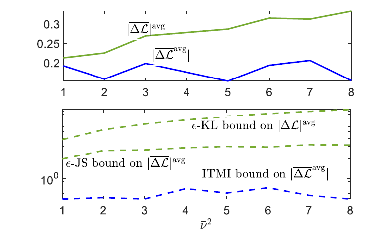
We also study examples where the obtained bound can be evaluated analytically or numerically. For the example of ridge regression with meta-learned bias, we illustrate the impact of task dissimilarity parameter on the two performance metrics, and their corresponding upper bounds,  in the following figure. As can be seen, while the absolute average meta-generalization gap metric appears to be largely insensitive to task dissimilarity, our metric reveals the role of task similarity, as captured by the bounds derived in the paper.

Problem

Machine learning models have become a ubiquitous tool for inference in various end-user applications such as natural language processing, face recognition and mobile healthcare management. In such highly personalized cases, it is important for the model to be able to adapt to the unique features of an individual with only a minimal amount of training data. Furthermore, the devices for which these personalized inference problems are relevant are typically power and/or memory constrained which limits the size of the model that can be used for learning on the edge.

Solution

In our recent work, accepted for publication in DSLW 2021, we focus on a solution using spiking neural networks (SNNs) that leverages the popular model agnostic meta-learning method to train a model that performs online inference while concurrently improving its ability to adapt to new tasks (termed online-within-online meta-learning (OWOML)-SNN). This meta-training method learns a hyperparameter initialization that can be quickly adapted to new tasks from a certain family as opposed to the standard paradigm in which a large ‘universal’ model is fixed at deployment. Biologically inspired SNN models that operate on sparse binary signals, are known to provide benefits in terms of energy efficiency, especially (as in our case) where a local learning rule would allow it to be implemented on a neuromorphic edge processor such as Intel’s Loihi chip.

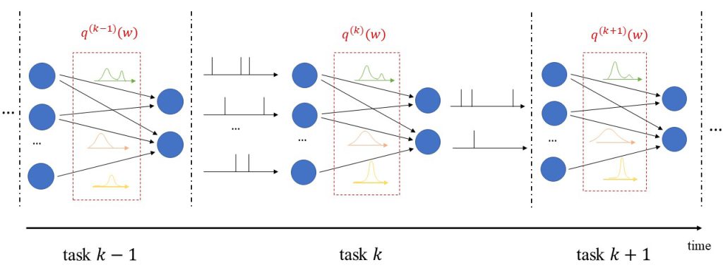
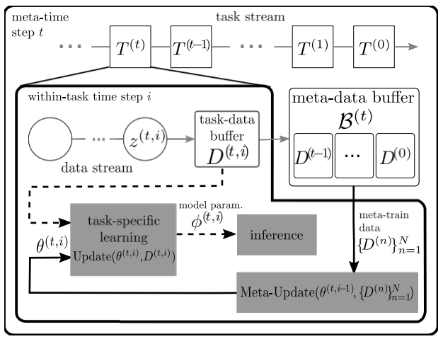
As show in Fig. 1, the proposed system assumes a stream of tasks for the SNN to adapt to, with streaming within-task data that it can learn from for online inference. Data from past tasks is stored in a fixed size buffer to be used for the meta-learning update. When new data for the current task arrives, multiple SNNs are instantiated using the hyperparameter initialization. One of those SNNs is used for online learning and inference while the others implement the meta-learning update to the hyperparameter initialization for use in the next iteration.

Results

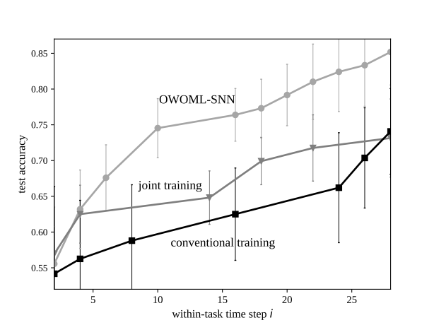
The performance of OWOML-SNN is compared to conventional per-task training and joint training. Under conventional training, a single SNN model is randomly initialized and learns only from the data available for the current task to perform online inference. Under joint training the SNN learns a so called ‘universal’ initialization by standard training across all previous tasks and then does per-task adaptation. We consider the family of omniglot character 2-way classification tasks with rate encoding to test the within-task generalization capabilities of our meta-learner.

The results in Fig. 2 for test accuracy over training at convergence of the hyperparameter initialization and joint training initialization show that the meta-learned initialization enables the fastest online adaptation of the three, providing an improvement in accuracy over conventional training that is about 18% larger that that of joint training after training on 5 examples from each class.

Please see our paper for further details.

Bleema Rosenfeld

Or how to remotely classify data with 80% accuracy and zero latency at Signal-to-Noise Ratios (SNRs) as low as – 8 dB.

Problem
The development of Internet of Things (IoT) systems, with applications ranging from personal healthcare and wearable devices to drone-based monitoring, is driving research efforts on edge-based machine learning. In such systems, data may be collected by battery-powered sensors and processed at a remote device, which may itself be energy-constrained. Standard hardware implementations pose major energy and latency limitations for such applications.
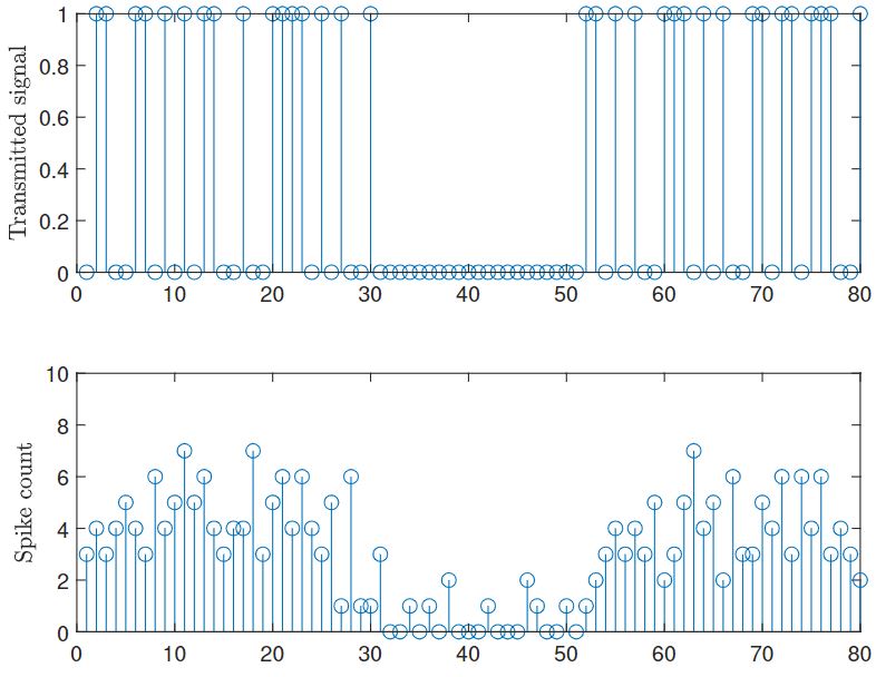
In our new paper, recently accepted at Asilomar 2020, we investigate a novel solution based on neuromorphic sensors, processors, and transmitter/receivers. In neuromorphic sensors, spikes (i.e., binary signals) mark the occurrence of a relevant event, e.g., a significant change in a pixel for a neuromorphic camera. Extremely low energy is consumed when the monitored scene is idle. In neuromorphic processors, known as Spiking Neural Networks (SNNs), spiking signals are processed via dynamic neural models for the detection of spatio-temporal patterns. SNNs have recently emerged as a biologically plausible alternative to ANNs, with significant benefits in terms of energy efficiency and latency. Finally, for communications, pulses, or spikes, can encode information for radio signalling via low-power Impulse Radio (IR). Commercial products are available for all these blocks, including DVS cameras, Intel’s Loihi SNN chip, and transceivers implementing the IEEE 802.15.4z IR standard.

System model
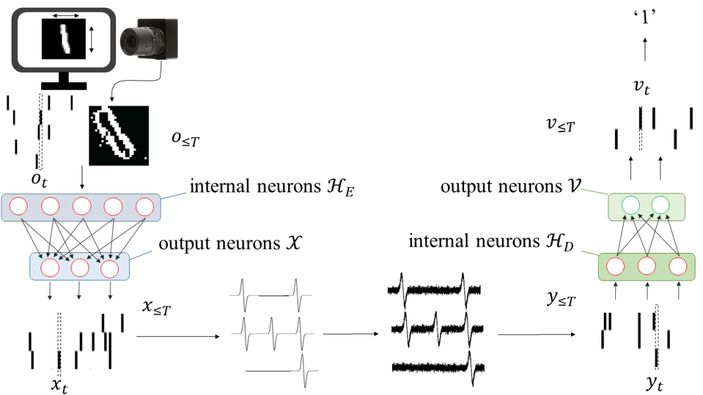
As seen in Fig. 1, the proposed system consists of the integration of neuromorphic sensing and processing with IR transmission, and it carries out Joint Source-Channel Coding (JSCC), as it performs source and channel coding in a single step. The signal sensed by the neuromorphic sensor, e.g., a DVS camera, is encoded as a vector of binary spiking signals, and processed by an encoding SNN that performs source and channel coding. The SNN defines a probabilistic mapping that is defined by its parameter vector. The output of the encoding SNN is modulated using parallel IR transmissions, with each spike encoded by an IR waveform such as a Gaussian monopulse. The channel is modeled as a frequency-flat Gaussian channel. Finally, the received signals are classified via a decoding SNN whose output can be interpreted as a class index using standard methods for SNN-based classification. For example, rate decoding predicts a class by selecting the neurons in an output layer with the largest number of spikes.
The proposed system in Fig. 1, termed NeuroJSCC, is trained by maximizing the log-likelihood that the decoding SNN outputs desired spiking signals in response to a given input. Details on the training procedure, and the resulting algorithm, can be found in the preprint.

Experiments

To illustrate the advantage of the system, we focus on an example consisting of the remote detection of handwritten digits recorded by a neuromorphic camera.
We compare NeuroJSCC to two benchmark schemes:
1) Uncoded transmission: The observation is directly transmitted through the Gaussian channel using On-Off Shift Keying (OOK), and classified using an SNN.
2) Separate Source-Channel Coding (SSCC): The encoder applies state-of-the-art quantization based on the Vector Quantization Variational Autoencoder (VQ-VAE) scheme, followed by LDPC encoding. The spiking signal is encoded as frames, and the scheme is applied separately to each one of them. At the decoder side, frames are decoded using the Belief Propagation algorithm, decompressed using VQ-VAE decoding, and then classified. We consider two different classifiers, namely traditional ANN and SNN.
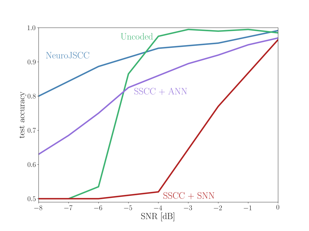
In Fig. 3, we evaluate the test accuracies at convergence obtained for different levels of SNR and the different schemes. The accuracy of Uncoded transmission drops sharply at sufficiently low SNR levels. In contrast, NeuroJSCC maintains a test accuracy of 80%, even at an SNR level as low as −8 dB. Separate SCC with an SNN as classifier suffers the most from the degradation of the SNR. Using an ANN proves more robust to low SNR levels, since an ANN can benefit from the non binary outputs of the VQ-VAE decoder without further loss of information due to binary quantization.
We refer to the main text for further experiments and analysis.
Code will be released shortly on our Github page.

Figure 1: Parameter Server (PS) computing architecture.

Problem Overview:

In order to scale machine learning so as to cope with large volumes of input data, distributed implementations of gradient-based methods, e.g., Gradient Descent (GD), that leverage the parallelism of first-order optimization techniques are commonly adopted. To run GD, as illustrated in Fig.~\ref{fig:model}, multiple parallel workers perform computations of the gradients and the Parameter Server (PS) iteratively aggregates the computed gradients and communicates the updated parameter back to the workers. In the process, the PS computing architecture is subject to two key impairments. First, the potentially high tail of the distribution of the computing times at the workers can cause significant slowdowns in wall-clock run-time per iteration due to straggling workers. Second, the communication overhead resulting from intensive two-way communications between the PS and the workers may require significant networking resources to be available in order not to dominate the overall run-time.

To jointly address these impairments, in a recent work just published on IEEE Transactions on Neural Networks and Learning Systems, we study the performance of coding and lazy aggregation techniques for the PS architecture in terms of wall-clock run-time complexity, communication complexity, and computation complexity.

Main Results:

To explore the trade-off among wall-clock time, communication, and computation requirements, we provide a unified analysis of the techniques of gradient coding (GC), worker grouping, and adaptive worker selection, also known as Lazily Aggregated Gradient (LAG), whose relative merits are summarized in Table I. Both GC and grouping are full-gradient approaches that aim at increasing robustness to stragglers by leveraging storage and computation redundancy. Thanks to coding, with GC, only a given number of workers, dependent on the computing redundancy, need to finish their computations and send their encoded computed gradients to the PS at each iteration in order to retrieve the gradient. Grouping applies data duplication and coding to groups of workers. In contrast, LAG is an approximate gradient descent scheme that judiciously selects a subset of active workers at each iteration in order to reduce communication and computation loads. By integrating all the techniques,
we propose a novel strategy, named Lazily Aggregated Gradient Coding (LAGC), that aims at exploring the trade-off between the robustness to stragglers of GC and the computation and communication efficiency of LAG by generalizing both schemes.

Figure 2: Time, communication, and computation complexity measures under the Pareto distribution.

Figure 3: Time, communication, and computation complexity measures under the exponential distribution.

As a special case, we also introduce a scheme that only uses grouping and adaptive selection, which is referred to as G-LAG. For illustration, we consider a linear regression model under two representative distributions, i.e., Pareto distribution and exponential distribution, accounting high- and low-tails for the distribution of the computing times for the workers. Time, communication and computation complexities of the existing strategies, namely GD, GC, and LAG, and the proposed strategies, i.e., LAGC and G-LAG, are shown in Fig. 2 and Fig. 3. It can be seen that both of the proposed LAGC and G-LAG are capable of combining the benefits of gradient coding and grouping in terms of robustness to stragglers with the communication and computation load gains of adaptive selection (see Table I). Furthermore, G-LAG provides the best wall-clock time and communication performance, while maintaining a low computational cost.
The full paper can be found here.

Welcome to King’s Centre for Learning and Information processing research blog.

We’re excited to share with you our findings in the future!