Category: meta-learning

Learning to Learn How to Calibrate

As discussed in our previous post ‘Is Accuracy Sufficient for AI in 6G? (No, Calibration is Equally Important)’, reliable AI should be able to quantify its uncertainty, i.e., to “know when it knows” and “know when it does not know”. To obtain reliable, or well-calibrated, AI models, two types of approaches can be adopted: (i) training-based calibration, and (ii) post-hoc calibration. Training-based calibration modifies the training procedure by accounting for calibration performance, and includes methods such as Bayesian learning [1, 2], robust Bayesian learning [3, 4], and calibration-aware regularization [5]; while post-hoc calibration utilizes validation data to “recalibrate” a probabilistic model, as in temperature scaling [6], Platt scaling [7], and isotonic regression [8]. All these methods have no formal guarantees on calibration, either due to inevitable model misspecification [9], or due to overfitting to the validation set [10, 11]. In contrast, conformal prediction (CP) offers formal calibration guarantees, although calibration is defined in terms of set, rather than probabilistic, prediction [12]. 

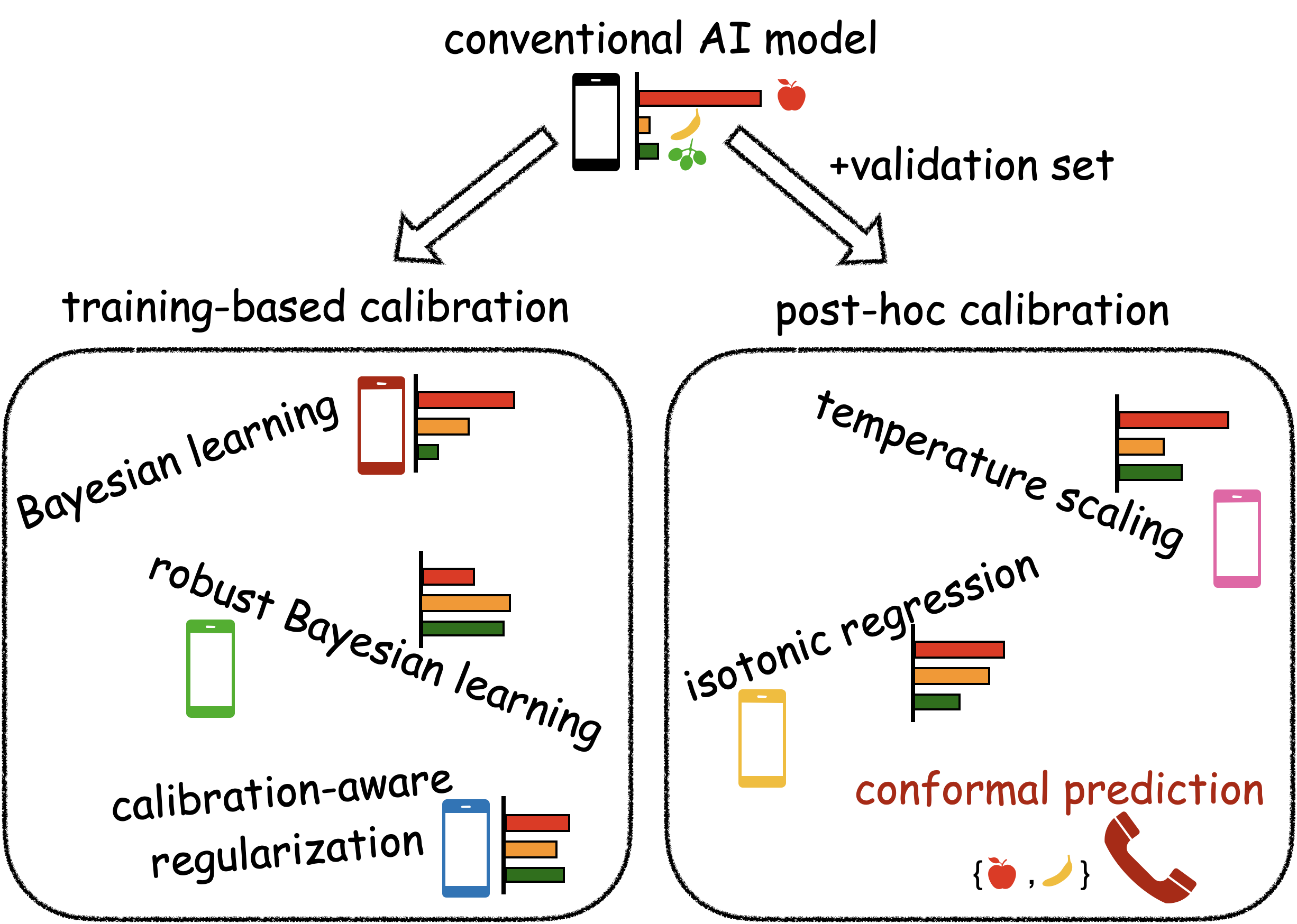
Fig. 1. Improvements in calibration can be obtained by either (i) training-based calibration or (ii) post-hoc calibration. Only conformal prediction, a post-hoc calibration approach, provides formal guarantees on calibration via set prediction.

A well-calibrated set predictor is the one that contains the true label with probability no smaller than a predetermined coverage level, say 90%. A set predictor obtained by conformal prediction is provably well calibrated, irrespective of the unknown underlying ground-truth distribution as long as the data examples are exchangeable, or i.i.d. (independent and identically distributed). 

One could trivially build a well-calibrated set predictor by producing the entire label set as the predicted set. However, such set predictor would be completely uninformative, since the size of the set predictor determines how informative the set predictor is. While conformal prediction is always guaranteed to yield reliable set predictors, it may produce large predicted set size in the presence of limited data examples [13]. In our recent work, presented at the NeurIPS 2022 Workshop on Meta-Learning, we have introduced a novel method that enhances the informativeness of CP-based set predictors via meta-learning.

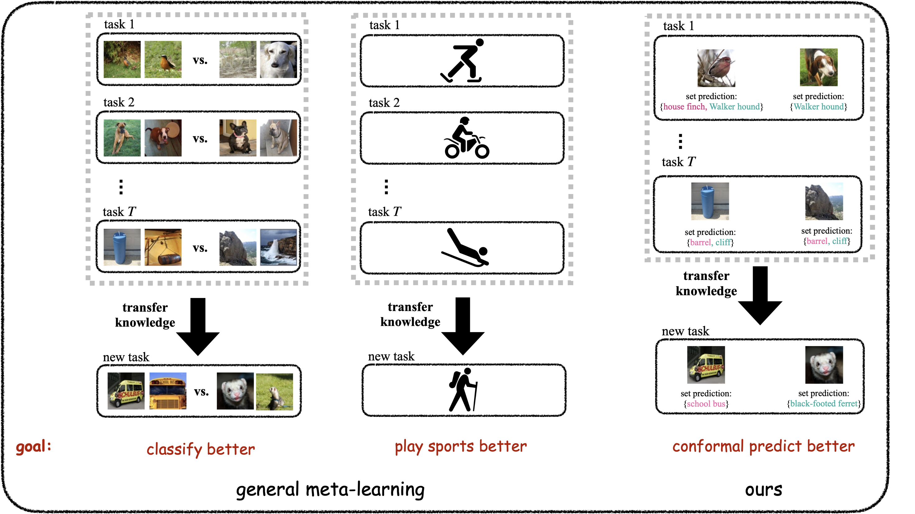
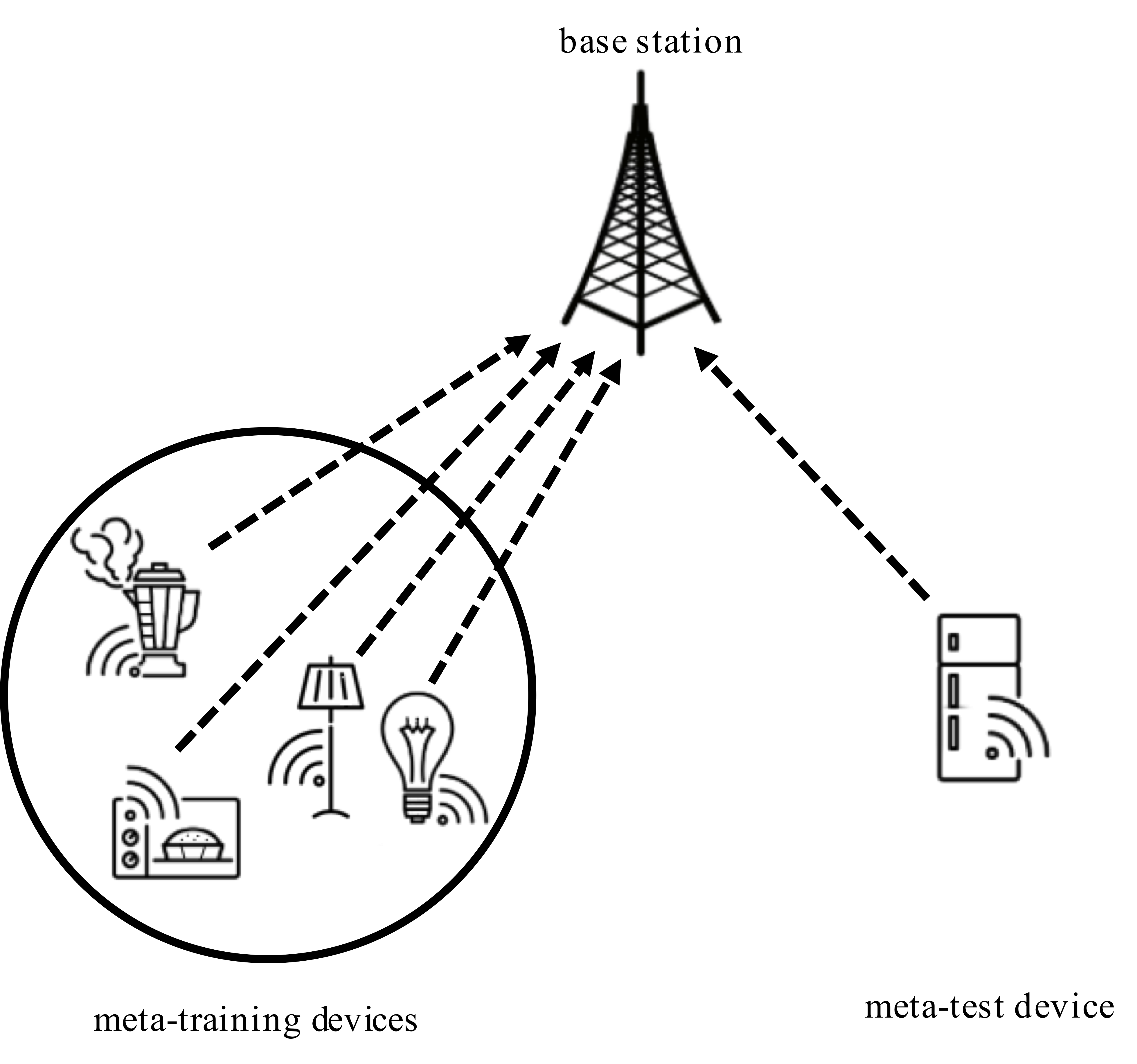
Fig. 2. Meta-learning transfers knowledge from multiple tasks. In our recent paper, we have proposed an application of meta-learning to conformal prediction with the aim of reducing the average prediction set size while preserving formal calibration guarantees.

Meta-learning, or learning to learn, transfers knowledge from multiple tasks to optimize the inductive bias (e.g., the model class) for new, related, tasks [14]. In our recent work, meta-learning was applied to cross-validation-based conformal prediction (XB-CP) [13] to achieve well-calibrated and informative set predictors. As demonstrated in the following figure, the proposed meta-learning approach for XB-CP, termed meta-XB, can reduce the average prediction set size as compared to conventional CP approaches (XB-CP and validation-based conformal prediction (VB-CP) [12]) and to previous work on meta-learning for VB-CP [14], while preserving the formal guarantees on reliability (the predetermined coverage level, 90%, is always satisfied for meta-XB). 

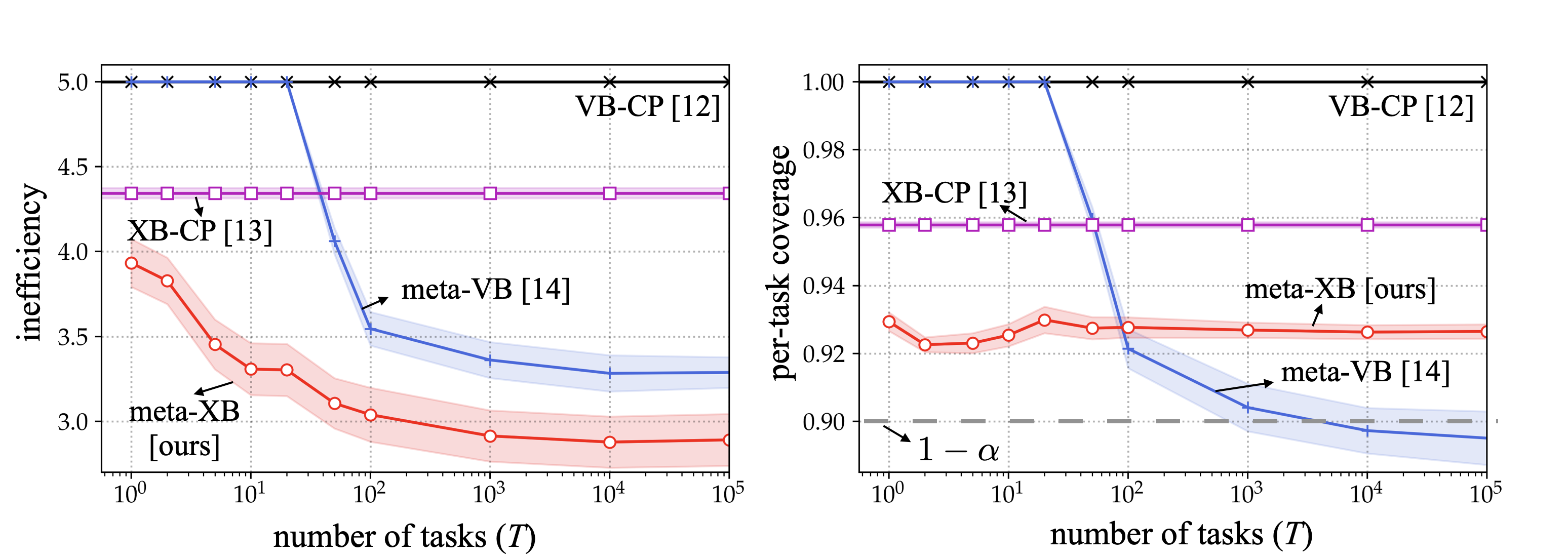
Fig. 3. Average prediction set size (left) and coverage (right) for new tasks as a function of number of meta-training tasks. As compared to conventional CP schemes (VB-CP and XB-CP), meta-learning based approaches (meta-VB and meta-XB) have smaller prediction set size; while the proposed meta-XB guarantees reliability for every task unlike meta-VB that satisfies coverage condition on average over multiple tasks.

For more details including improvements in terms of input-conditional coverage via meta-learning with adaptive nonconformity scores [15], and further experimental results on image classification and communication engineering aspects, please refer to the arXiv posting.

References

[1] O. Simeone, Machine learning for engineers. Cambridge University Press, 2022

[2] J. Knoblauch, et al, “Generalized variational inference: Three arguments for deriving new posteriors,” arXiv:1904.02063, 2019

[3] W. Morningstar, et al “PACm-Bayes: Narrowing the empirical risk gap in the Misspecified Bayesian Regime,” NeurIPS 2021

[4] M. Zecchin, et al, “Robust PACm: Training ensemble models under model misspecification and outliers,” arXiv:2203.01859, 2022

[5] A. Kumar, et al, “Trainable calibration measures for neural networks from kernel mean embeddings,” ICML 2018

[6] C. Guo, et al, “On calibration of modern neural networks,” ICML 2017

[7] J. Platt, et al, “Probabilistic outputs for support vector machines and comparisons to regularized likelihood method,” Advances in Large Margin Classifiers 1999

[8]  B. Zadrozny and C. Elkan “Transforming classifier scores into accurate multiclass probability estimates,” KDD 2022

[9] A. Masegosa, “Learning under model misspecification: Applications to variational and ensemble methods.” NeurIPS 2020

[10] A. Kumar, et al, “Verified Uncertainty Calibration,” NeurIPS 2019

[11] X. Ma and M. B. Blaschko, “Meta-Cal: Well-controlled Post-hoc Calibration by Ranking,” ICML 2021 

[12]  V. Vovk, et al, “Algorithmic Learning in a Random World,” Springer 2005

[13] R. F. Barber, et al, “Predictive inference with the jackknife+,” The Annals of Statistics, 2021

[14] Chen, Lisha, et al. “Learning with limited samples—Meta-learning and applications to communication systems.” arXiv preprint arXiv:2210.02515, 2022.

[14] A. Fisch, et al, “Few-shot conformal prediction with auxiliary tasks,” ICML 2021

[15] Y. Romano, et al, “Classification with valid and adaptive coverage,” NeurIPS 2020


Is Accuracy Sufficient for AI in 6G? (No, Calibration is Equally Important)

AI modules are being considered as native components of future wireless communication systems that can be fine-tuned to meet the requirements of specific deployments [1]. While conventional training solutions target the accuracy as the only design criterion, the pursuit of “perfect accuracy” is generally neither a feasible nor a desirable goal. In Alan Turing’s words, “if a machine is expected to be infallible, it cannot also be intelligent”. Rather than seeking an optimized accuracy level, a well-designed AI should be able to quantify its uncertainty: It should “know when it knows”, offering high confidence for decisions that are likely to be correct, and it should “know when it does not know”, providing a low confidence level for decisions are that are unlikely to be correct. An AI module that can provide reliable measures of uncertainty is said to be well-calibrated.

Importantly, accuracy and calibration are two distinct criteria. As an example, Fig. 1 illustrates  a QPSK demodulator trained using limited number of pilots. Depending on the input, the trained probabilistic model may result in either accurate or inaccurate demodulation decisions, whose uncertainty is either correctly or incorrectly characterized.

Fig. 1. The hard decision regions of an optimal demodulator (dashed lines) and of a data-driven demodulator trained on few pilots (solid lines) are displayed in panel (a), while the corresponding probabilistic predictions for some outputs are shown in panel (b).


The property of “knowing what the AI knows/ does not know” is very useful when the AI module is used as part of a larger engineering system. In fact, well-calibrated decisions should be treated differently depending on their confidence level. Furthermore, well-calibrated models enable monitoring – by tracking the confidence of the decisions made by an AI – and other functionalities, such as anomaly detection [2].

In a recent paper from our group published on the IEEE Transaction on Signal Processing [3], we proposed a methodology to develop well-calibrated and efficient AI modules that are capable of fast adaptation. The methodology builds on Bayesian meta-learning.

To start, we summarize the main techniques under consideration.

  1. Conventional, frequentist, learning ignores epistemic uncertainty – uncertainty caused by limited data – and tends to be overconfident in the presence of limited training samples.
  2. Bayesian learning captures epistemic uncertainty by optimizing a distribution in the model parameter space, rather than finding a single deterministic value as in frequentist learning. By obtaining decisions via ensembling, Bayesian predictors can account for the “opinions” of multiple models, hence providing more reliable decisions. Note that this approach is routinely used to quantify uncertainty in established fields like weather prediction [4].
  3. Frequentist meta-learning [5], also known as learning to learn, optimizes a shared training strategy across multiple tasks, so that it can easily adapt to new tasks. This is done by transferring knowledge from different learning tasks. As a communication system example, see Fig. 2 in which the demodulator adapts quickly with only few pilots for a new frame. While frequentist meta-learning is well-suited for adaptation purpose, its decisions tend to be overconfident, hence not improving monitoring in general.
  4. Bayesian meta-learning [6,7] integrates meta-learning with Bayesian learning in order to facilitate adaptation to new tasks for Bayesian learning.
  5. Bayesian active meta-learning [8] Active meta-learning can reduce the number of meta-training tasks. By considering streaming-fashion of availability of meta-training tasks, e.g., sequential supply of new frames from which we can online meta-learn the AI modules, we were able to effectively reduce the time required for satisfiable meta-learning via active meta-learning.


Fig. 2. Through meta-learning, a learner (e.g., demodulator) can be adapted quickly using few pilots to new environment, using hyperparameter vector optimized over related learning tasks (e.g., frames with different channel conditions).


Some Results

We first show the benefits of Bayesian meta-learning for monitoring purpose by examining the reliability of its decisions in terms of calibration. In Fig. 3, reliability diagrams for frequentist and Bayesian meta-learning are compared. For an ideal calibrated predictor, the accuracy level should match the self-reported confidence (dashed line in the plots). In can be easily checked that AI modules designed by Bayesian meta-learning (right part) are more reliable than the ones with Frequentist meta-learning (left part), validating the suitability of Bayesian meta-learning for monitoring purpose. Experimental results are obtained by considering a demodulation problem.


Fig. 3. Bayesian meta-learning (right) yields reliable decisions as compared to frequentist meta-learning (left) which can be captured via reliability diagrams [9].

Fig. 4 demonstrates the impact of Bayesian active meta-learning that successfully reduces the number of required meta-training tasks. The results are obtained by considering an equalization problem.

Fig. 4. Bayesian active meta-learning actively searches for meta-training tasks that are most surprising (left), hence increasing the task efficiency as compared to Bayesian meta-learning which randomly chooses tasks to be meta-trained.


References

[1] O-RAN Alliance, “O-RAN Working Group 2 AI/ML Workflow Description and Requirements,” ORAN-WG2. AIML. v01.02.02, vol. 1, 2.

[2] C. Ruah, O. Simeone, and B. Al-Hashimi, “Digital Twin-Based Multiple Access Optimization and Monitoring via Model-Driven Bayesian Learning,” arXiv preprint arXiv:2210.05582.

[3] K.M. Cohen, S. Park, O. Simeone and S. Shamai, “Learning to Learn to Demodulate with Uncertainty Quantification via Bayesian Meta-Learning,” arXiv https://arxiv.org/abs/2108.00785

[4] T. Palmer, “The Primacy of Doubt: From Climate Change to Quantum Physics, How the Science of Uncertainty Can Help Predict and Understand Our Chaotic World,” Oxford University Press, 2022.

[5] C. Finn, P. Abbeel, and S. Levine, “Model-Agnostic Meta-Learning for Fast Adaptation of Deep Networks,” in Proceedings of the 34th International Conference on Machine Learning, vol. 70. PMLR, 06–11 Aug 2017, pp. 1126–1135.

[6] J. Yoon, T. Kim, O. Dia, S. Kim, Y. Bengio, and S. Ahn, “Bayesian Model-Agnostic Meta-Learning,” Proc. Advances in neural information processing systems (NIPS), in Montreal, Canada, vol. 31, 2018.

[7] C. Nguyen, T.-T. Do, and G. Carneiro, “Uncertainty in Model-Agnostic Meta-Learning using Variational Inference,” in Proceedings of the IEEE/CVF Winter Conference on Applications of Computer Vision, 2020, pp. 3090–3100.

[8] J. Kaddour, S. Sæmundsson et al., “Probabilistic Active Meta-Learning,” Proc. Advances in Neural Information Processing Systems (NIPS) as Virtual-only Conference, vol. 33, pp. 20 813–20 822, 2020.

[9] C. Guo, G. Pleiss, Y. Sun, and K. Q. Weinberger, “On Calibration of Modern Neural Networks,” in International Conference on Machine Learning. PMLR, 2017, pp. 1321–1330.

Meta-learning: A new framework for few-pilot transmission in IoT networks

Problem

Fig. 1: Illustration of few-pilot training for an IoT system via meta-learning

For channels with an unknown model or an unavailable optimal receiver of manageable complexity, the design of demodulation and decoding can potentially benefit from a data-driven approach based on machine learning. Machine learning solutions, however, cannot be directly applied to Internet- of-Things (IoT) scenarios in which devices transmit sporadically using short packets with few pilot symbols. In fact, the few pilots do not provide enough data for training the receiver.

A Novel Solution based on Meta-learning

Fig. 2: MAML is to find an initial value 𝜃 that minimizes the loss L𝑘(θ´𝑘) for all devices 𝑘 after one step of update. In contrast, joint training carries out an optimization on the cumulative loss              L1(θ) + L2(θ) 

In a recent work to be presented at IEEE SPAWC 2019, we proposed a novel solution for demodulation in IoT networks that is based on model-agnostic meta-learning (MAML) algorithm. The key idea is to use pilots from previous transmissions of other IoT devices as meta- training data in order to learn a demodulator that is able to quickly adapt to the end-to-end channel conditions of a new device from few pilots. MAML derives an inductive bias as an initialization point for a neural network-based demodulator. As illustrated in Fig. 2, MAML seeks an initialization point such that all the performance losses of the demodulators for all IoT devices obtained after one update are collectively minimized. In comparison, a more conventional approach to use meta-training data, namely joint training, would pool together all the pilots received from the meta-training devices and seeks for minimizing the cumulative loss.

Some Results

To give a taste of the results in the paper, we now provide an example.

Fig. 3: Probability of symbol error with respect to number of pilots for the  meta-test device (see paper).

In Fig. 3, we plot probability of symbol error with respect to the number of pilots for new IoT device in offline scenario. We adopt 16-QAM with 100 meta-training devices, each with 32 pilots for meta-training. We compare the performance of state-of-the-art meta-learning approaches including MAML with: (i) a fixed initialization scheme where data from the meta-training devices is not used; (ii) joint training with the meta-training dataset as described above.

All of the various meta-learning schemes are seen to vastly outperform the mentioned baseline approaches (i) – (ii) by adapting to the channel of the meta-test device using only a few pilots. In contrast, joint training shows similar performance compared to fixed initialization. This confirms that, unlike conventional solutions, meta-learning can effectively transfer information from meta-training devices to a new target device.


Fig. 4: Average probability of symbol error with respect to average number of pilots over slots t=71, …, 90 for online meta-learning (see paper).

In Fig. 4, we plot probability of symbol error with respect to average number of pilots in online scenario. Through comparison with fixed initialization case, we have shown that proposed adaptive pilot number selection scheme can reduce pilot overhead with any online schemes. Moreover, when proposed scheme comes with online meta-learning, we show that pilot overhead is reduced even more under negligible performance degradation. This again confirms that meta-learning can acquire useful inductive bias from previous IoT devices.

The full paper can be found here.