An emerging research topic in artificial intelligence (AI) consists in designing systems that take inspiration from biological brains. This is notably driven by the fact that, although most AI algorithms become more and more efficient (for instance, for image generation), this comes at a cost. Indeed, with architectures constantly growing in size, training a single large neural network today consumes a prohibitive amount of energy. Despite consuming only about 12W, human brains exhibit impressive capabilities, such as life-long learning.
By taking a Bayesian perspective, we demonstrate in our latest work how biologically inspired spiking neural networks (SNNs) can exhibit learning mechanisms similar to those applied in brains, which allow them to perform continual learning. As we will see, the technique also solves a key challenge in deep learning, that is, to obtain well calibrated solutions in the face of previously unseen data.
Our work
Bayesian Learning
As seen in Fig. 1, we propose to equip each synaptic weight in the SNN with a probability distribution. The distribution captures the epistemic uncertainty induced by the lack of knowledge of the true distribution of the data. This is done by assigning probabilities to model parameters that fit equally well the data, while also being consistent with prior knowledge. As a consequence, Bayesian learning is known to produce better calibrated decisions, i.e., decisions whose associated confidence better reflects the actual accuracy of the decision.
This contrasts with frequentist learning, in which the vector of synaptic weights is optimized by minimizing a training loss. The training loss is adopted as a proxy for the population loss, i.e., for the loss averaged over the true, unknown, distribution of the data. Therefore, frequentist learning disregards the inherent uncertainty caused by the availability of limited training data, which causes the training loss to be a potentially inaccurate estimate of the population loss. As a result, frequentist learning is known to potentially yield poorly calibrated, and overconfident decisions for ANNs.
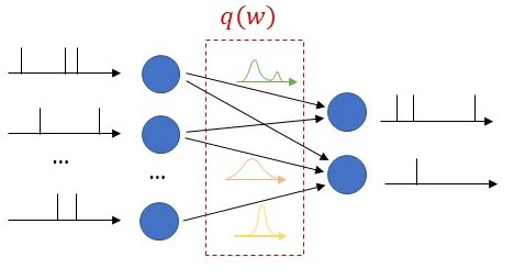
Figure 1: Illustration of Bayesian learning in an SNN: In a Bayesian SNN, the synaptic weights are assigned a joint distribution, often simplified as a product distribution across weights.
We consider both real-valued (with possibly limited resolution, as dictated by deployment on neuromorphic hardware) and binary-valued synapses, parametrised by Gaussian and Bernoulli distributions, respectively. The advantages of models with binary-valued synapses, i.e., binary SNNs, include a reduced complexity for the computation of the membrane potential. Furthermore, binary SNNs are particularly well suited for implementations on chips with nanoscale components that provide discrete conductance levels for the synapses.
Continual Learning
In addition to uncertainty quantification, we apply the proposed solution to continual learning, as illustrated in Fig. 2. In continual learning, the system is sequentially presented several datasets corresponding to distinct, but related, learning tasks, where each task is selected, possibly with replacement, from a pool of tasks, and its identity is unknown to the system. Its goal is to learn to make predictions that generalize well each new task, while causing minimal loss of accuracy on previous tasks.
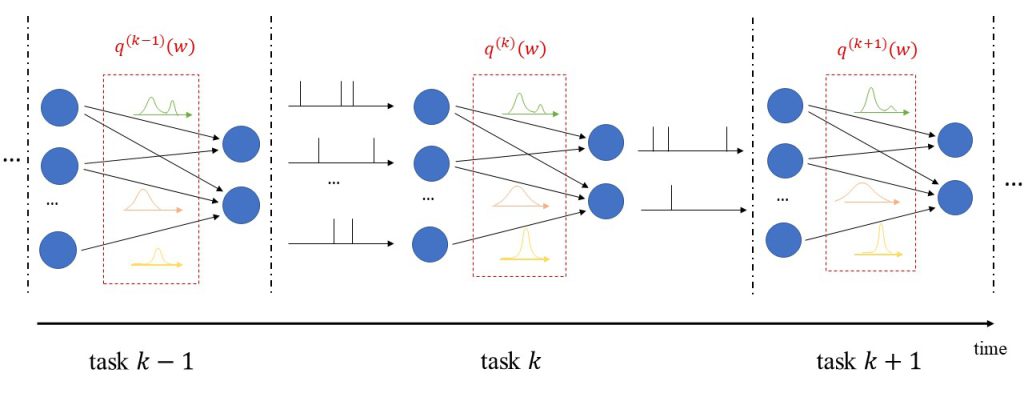
Figure 2: Illustration of Bayesian continual learning: the system is successively presented with similar, but different, tasks. Bayesian learning allows the model to retain information about previously learned information.
Many existing works on continual learning draw their inspiration from the mechanisms underlying the capability of biological brains to carry out life-long learning. Learning is believed to be achieved in biological systems by modulating the strength of synaptic links. In this process, a variety of mechanisms are at work to establish short-to intermediate-term and long-term memory for the acquisition of new information over time. These mechanisms operate at different time and spatial scales.
Biological Principles of Learning
One of the best understood mechanisms, long-term potentiation, contributes to the management of long-term memory through the consolidation of synaptic connections. Once established, these are rendered resistant to disruption by changing their capacity to change via metaplasticity. As a related mechanism, return to a base state is ensured after exposition to small, noisy changes by heterosynaptic plasticity, which plays a key role in ensuring the stability of neural systems. Neuromodulation operates at the scale of neural populations to respond to particular events registered by the brain. Finally, episodic replay plays a key role in the maintenance of long-term memory, by allowing biological brains to re-activate signals seen during previous active periods when inactive (i.e., sleeping).
In this work, we demonstrate how the continual learning rule we obtain exhibits some of these mechanisms. In particular, synaptic consolidation and metaplasticity for each synapse can be modeled by a precision parameter. A larger precision reduces the step size of the synaptic weight updates. During learning, the precision is increased to the degree that depends on the relevance of each synapse as measured by the estimated Fisher information matrix for the current mini-batch of examples.
Heterosynaptic plasticity, which drives the updates towards previously learned and resting states to prevent catastrophic forgetting, is obtained from first principles via an information risk minimization formulation with a Kullback-Leibler regularization term. This mechanism drives the updates of the precision and mean parameter towards the corresponding parameters of the variational posterior obtained at the previous task.
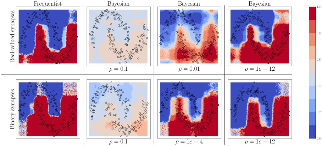
Figure 3: Predictive probabilities evaluated on the two-moons dataset after training for Bayesian learning. Top row: Real-valued synapses; Bottom row: Binary synapses.
Results
We start by considering the two-moons dataset shown in Fig. 3. Triangles indicate training points for a class “0’’, while circles indicate training points for a class “1”. The color intensity represents the predictive probabilities for frequentist learning and for Bayesian learning: the more intense the color, the higher the prediction confidence determined by the model. Bayesian learning is observed to provide better calibrated predictions, that are more uncertain outside the input regions covered by training data points. As can be seen, confidence for the Bayesian models can be mitigated by a parameter, as precised in the full text.

Figure 4: Top three classes predicted by both Bayesian and frequentist models on selected examples from the DVS-Gestures dataset. Top: real-valued synapses. Bottom: binary synapses. The correct class is indicated in bold font.
This point is further illustrated in Fig. 4 by showing the three largest probabilities assigned by the different models on selected examples from DVS-Gestures dataset, considering real-valued synapses in the top row and binary synapses in the bottom row. In the left column, we observe that, when both models predict the wrong class, Bayesian SNNs tend to do so with a lower level of certainty, and typically rank the correct class higher than their frequentist counterparts. Specifically, in the examples shown, Bayesian models with both real-valued and binary synapses rank the correct class second, while the frequentist models rank it third. Furthermore, as seen in the middle column, in a number of cases, the Bayesian models manage to predict the correct class, while the frequentist models predict a wrong class with high certainty. In the right column, we show that even when frequentist models predict the correct class and Bayesian models fail to do so, they still assign lower probabilities (i.e., <50%) to the predicted class.
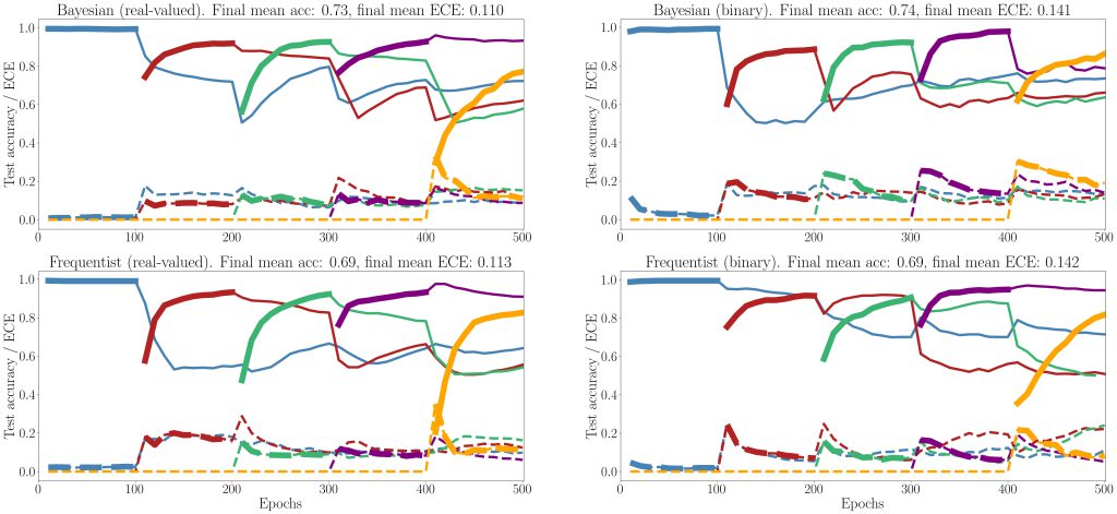
Figure 5: Evolution of the average test accuracies and ECE on all tasks of the split-MNIST-DVS across training epochs, with Gaussian and Bernoulli variational posteriors, and frequentist schemes for both real-valued and binary synapses. Continuous lines: test accuracy, dotted lines: ECE, bold: current task. Blue: {0, 1}; Red: {2, 3}; Green: {4, 5}; Purple:{6, 7}; Yellow: {8, 9}.
Finally, we show results for continual learning on the MNIST-DVS dataset in Fig. 5. We show the evolution of the test accuracy and expected calibration error (ECE) on all tasks, represented with lines of different colors, during training. The performance on the current task is shown as a thicker line. We consider frequentist and Bayesian learning, with both real-valued and binary synapses. With Bayesian learning, the test accuracy on previous tasks does not decrease excessively when learning a new task, which shows the capacity of the technique to tackle catastrophic forgetting. Also, the ECE across all tasks is seen to remain more stable for Bayesian learning as compared to the frequentist benchmarks. For both real-valued and binary synapses, the final average accuracy and ECE across all tasks show the superiority of Bayesian over frequentist learning.
More details can be found in the full text at this link.

Leave a Reply