
Last time out, I discussed options for replicating findings from a genome-wide association study when no appropriate cohort exists for replication. Perhaps the most effective solution was time – wait for more samples, get more power and prove those pesky doubters wrong. As all good sci-fi fans know (and as all bad sci-fi fans definitely know) time is a two-way street, and so in this blog, I’ll look back in time to explore the early strength of association of genetic regions that would later be classified as genome-wide significant.

To this end, let us turn once again to the treasure trove of open genomic data that is the Psychiatric Genomics Consortium, or PGC. For several years, the PGC has been creating world-wide collaborations to perform large genome-wide association studies of psychiatric disorders, and (crucially) making the results openly-accessible to all via a downloads page. Seriously – click that link, go to the page. Provided you agree not to use the results to compete with the primary role of the PGC (finding genomic regions associated with psychiatric disorders), you can download results and explore them to your heart’s content.
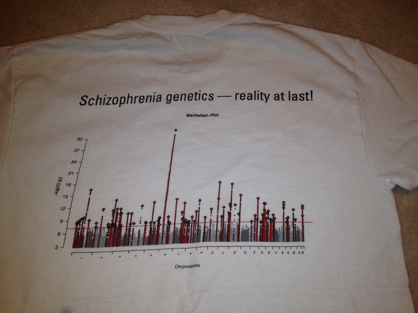
From that page, we can download two sets of statistics. First, the PGC2 2014 Schizophrenia results. These were kind of a big deal, because they compared 36,989 cases and 113,075 controls and identified 108 regions strongly associated with schizophrenia. That is, the association with these variants had p-values lower than the level set for genome-wide significance, p< 5 x 10⁻⁸, which effectively Bonferroni corrects a standard p value of 0.05 for one million tests. Finding 108 genome-wide significant hits was a huge increase, and made researchers very excited, sufficiently so that there were t-shirts! You know you’ve made it big when there are t-shirts.
But the interesting part of today’s blog uses the PGC1 Schizophrenia results from 2011, which examined 9,394 cases and 12,462 controls (ignoring replication) and identified five regions associated with schizophrenia. The question is: where were the future significant regions in this earlier paper? If we look backwards from the 2014 paper findings, how do they look in the 2011 paper?
Let’s begin with standard replication where we look forwards rather than backwards. Of the five regions significantly associated in 2011, three were also associated in 2014. The exceptions were regions on chromosomes 8 (p-value of 1 x 10⁻⁷), which approached genome-wide significance and may yet replicate, and 11 (1 x 10⁻⁴), which was far further from significance in the 2014 paper, demonstrating the value of replication.
“where were the future significant regions in this earlier paper?”
So three regions from the 2014 paper were genome-wide significant in the 2011, and accounted for three out of five regions at that significance level. As such, the proportion of findings from the 2011 paper that remained genome-wide significant in the 2014 paper was 3/5 or 60%. Continuing this across all the 108 loci, we find that:
- 3 had p ≤ 5 x 10⁻⁸ (60% of regions at this level)
- 4 had p ≤ 5 x 10⁻⁷ (44% of regions at this level)
- 9 had p ≤ 5 x 10⁻⁶ (28% of regions at this level)
- 7 had p ≤ 5 x 10⁻⁵ (6% of regions at this level)
- 29 had p ≤ 5 x 10⁻⁴ (5% of regions at this level)
- 33 had p ≤ 5 x 10⁻³ (1% of regions at this level)
- 15 had p ≤ 5 x 10⁻² (0.5% of regions at this level)
- 4 had p > 5 x 10⁻²
- 4 regions were not represented (three on the X chromosome and one region that was just a single variant)
What does this tell us? It says that regions that will later reach significance in larger studies have low (i.e. approaching significant) p-values in earlier, smaller studies. Most of the 104 loci we could examine here had at least nominal (p<0.05) significance in the previous analysis. Regions of interest don’t emerge from nowhere. Even in studies not large enough to capture accurately the small effects of individual variants on psychiatric traits, future regions of importance still have low p-values. But crucially, most regions with low p-values (i.e. those approaching significance) do not go on to be supported, at least in the short term. While the signal is there, there’s a lot of noise as well, and this grows as higher p-values are considered (e.g. p ≤ 5 x 10⁻² where only 0.5% of regions remain significant).
“GWAS, like so much of science, is about building layers of evidence”
Exploring the regions below significance can be valuable, and this example taken alone suggests that focusing on regions with p < 5 x 10⁻⁶ may be a good starting point. However, we should always be aware that this is exploratory – most of the regions being discussed may not turn out to be truly interesting. GWAS, like so much of science, is about building layers of evidence – these studies are the floor of the palace of understanding: we can see where the rooms are going to go, but we need to build up studies to get to the roof. Otherwise we’ll get wet when it rains.
Note for serious geneticists: this analysis was quick and dirty, and any conclusions of import should be based on a far more robust investigation. I’m always happy to share my code and to identify where more rigour is required.