Quasi-experimental methods can be just as robust

By Henry Woodward, Quantitative Consultant at Stonehaven and Chiamaka Nwosu, Data and Research Analyst at King’s College London

It is a commonly held misconception that quasi experimental methods are not as good as experimental methods such as Randomised Controlled Trials (RCTs). Quasi experimental analysis can be just as robust at establishing a causal link between a program and an impact as running an experimental trial. There are several types of quasi-experimental methods, however this blog will discuss the two most frequently used. The regression discontinuity design (RDD) and the difference-in-differences (DID) method.

What is the RDD and DID method?

Regression Discontinuity Designs (RDD) and the Difference-in-Differences (DID) method are examples of quasi-experimental research designs. The RDD uses a cut-off to determine the assignment of an intervention and its causal impact, while the DID estimates causality by calculating the differential effects between two distinct groups at multiple time periods[i]. There are benefits and limitations to using either, and the decision on which method to use is largely driven by the data available.

When implemented properly, the RDD yields an unbiased estimate of the local treatment effect

An RDD allows for a comparison of similar students on opposite sides of a certain threshold. For example, students who are narrowly above the arbitrary threshold for a bursary shouldn’t have latent differences compared to those who fall just below such a threshold – yet one receives a bursary and one doesn’t. After controlling for observable differences, you can assume the differences in outcome measure can be attributed to the treatment – the bursary (see Figure 1.)

The RDD has several advantages including but not limited to the following:

• When well implemented and analysed, RDD yields an unbiased estimate of the local treatment effect[ii].
• The RDD can generate treatment effect estimates like those from RCTs [iii].
• And does not require ex-ante randomisation (i.e. randomisation prior to the intervention) which avoids some of the ethical issues associated with random assignment.

Three main limitations of the RDD

The first limitation is that the estimated effects of an RDD are only unbiased if the relationship between the treatment allocation variable and outcome variable is modelled correctly. E.g. a linear model should not be used to model a non-linear relationship and vice versa[iv]. Another limitation is that an RDD will outline the effect of the treatment for individuals who are near the arbitrary threshold for treatment allocation, and not those who are further from that threshold[v]. Coming back to our bursary example, whilst a RDD could show the impact of the bursary for those in and around the income level required to qualify for the bursary on whichever outcome measure, it does not show what impact a bursary has on the same outcome measure for those who fall way below this income level. This may make evaluating an intervention harder as frequently the extreme cases are often those specifically targeted by an intervention.

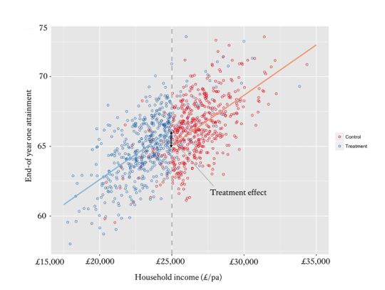
 Figure 1. A regression discontinuity demonstrating the impact of bursaries on end-of year attainment. [vi]

[i] Students whose household income falls below £25,000pa are eligible for a King’s bursary, whilst those whose household income falls above £25,000pa are not.  Comparing the constants at this threshold when regressing household income on end-of year attainment for those above and below the £25,000pa threshold provides an unbiased estimate of the impact of bursaries on attainment.  

There are also some practical limitations to consider. Firstly, because analysis uses observations close to an arbitrary threshold, the sample size can often be too small that it fails to have the power to uncover significant effects[1] This is particularly problematic for WP teams that run multiple interventions on a small number of potential students, contamination by other treatment can confound results. If treatment allocations on other initiatives employ the same arbitrary cut-off, then the discontinuity may be partially (or totally) explained by other treatments. To use the bursary example again, if you wanted to estimate the impact of the bursary, you could run an RDD on students falling just above and below the qualifying household income of (e.g. £25,000pa). However, it could also be the case that being below the £25,000pa cut-off qualifies for a travel pass, discounts on learning materials, and free extra tuition. In this instance, you would not know whether the discontinuity in outcome measure was due to the bursary or these other treatments.

Difference-in-Differences is another important quasi – experimental method

The DID method relies on the existence of two groups and multiple time periods, such that comparing the difference between the two differences is the effect of the intervention. The difference-in-differences estimator is the difference in average outcome of a treatment group before and after the intervention minus the difference of the comparator group over the same period.

Thinking about the bursary example, if we assume that there were national changes to bursary policies which will be implemented by universities at different points in the year. We could compare the effect on, average grades for students in two universities of interest, before and after the policy was implemented (see Table 1). In this case, the treatment would be the modified bursary policy. The effect of the intervention is calculated as: Difference = Endline grades (Y1) – Baseline grades (Y1) – Endline grades (Y0) – Baseline grades (Y0)  i.e. (78-64) – (53-58) = 14 – (-5) =19.

	Baseline grades	Endline grades	Change
Treatment (Y1)	64	78	14
Comparison (Y0)	58	53	-5
Difference	–	25	19

Table 1. Average grades

The methodology improves on treatment estimators based on comparing differences in your outcome measure for exclusively your participants pre- and post-intervention (pre-/post-test) as this will be biased if there is a natural trend in outcome measure over the same time period. Additionally, it improves on estimators based on differences between participants and a comparator group exclusively post-intervention as this will be biased if there are natural differences between groups.

Limitations of Difference-in-differences

One limitation to difference-in-differences methodology is that it requires repeated measures (including a baseline) which rules out its use for outcome data that can only be collected once. It also requires the construction of a non-intervention comparator group. This isn’t too problematic for administratively collected data (such as A-levels or HE enrolment) providing you have been granted the consent to track non-participant individuals. However, it could be more complex for more bespoke outcome measures. As this requires the researcher to repeatedly collect data on participants not involved with the initiative (some of whom may not be thrilled about not being on the initiative in the first place).

The critical limitation to difference-in-difference analysis is the parallel trend assumption. This assumption specifies that the trend of outcome over time needs to be the same for the treatment and comparator groups in the absence of the intervention. However, this assumption cannot be directly tested[2]. A way around this is to acquire more data at time periods pre- and post-intervention to inspect the trend for the two groups, and go some way towards verifying the parallel trend assumption. Again, a logistical problem here is having to collect data at multiple points on both treatments and comparator groups.

In DID design it is crucial that the researcher examines the population composition of the treatment and comparator groups before and after the intervention to foster greater validity and to make sure there hasn’t been cross-contamination.

Quasi-experimental methods can sometimes be the best approach

As HE practitioners it is necessary to be able to demonstrate the impact of interventions we run. Although a randomised controlled trial is often the best way of establishing a causal link between a program and an impact, these can be difficult to implement. When having a control group could be harmful and randomisation is not possible. But, good quality, historical data is available,  quasi-experimental methods are the best approach to evaluate impact because they allow us to estimate the causal impact of a program without the complications of an experimental method.

_______________________________________________________________________

Read our reports

Click here to join our mailing list.

Follow us on Twitter: @KCLWhatWorks

_______________________________________________________________________

[i] Greene, W. H. (2012). Econometric Analysis. England: Pearson Education Limited.

[ii] Rubin, D. B. (1977), “Assignment to Treatment Group on the Basis of a Covariate,” Journal of Educational Statistics, 2, pp.34-58

[iii] Moss, B. G., Yeaton, W. H., & LIoyd, J. E. (2014). “Evaluating the effectiveness of developmental mathematics by embedding a randomized experiment within a regression discontinuity design”. Educational Evaluation and Policy Analysis, 36(2), pp.170-185.

[iv] Greene, W. H. (2012). Econometric Analysis. England: Pearson Education Limited.

[v] Ibid.

[vi] Students whose household income falls below £25,000pa are eligible for a King’s bursary, whilst those whose household income falls above £25,000pa are not.  Comparing the constants at this threshold when regressing household income on end-of year attainment for those above and below the £25,000pa threshold provides an unbiased estimate of the impact of bursaries on attainment.  

[vii] Reichardt C.S., Trochim W.M.K. & Cappelleri J.C. (1995) Reports of the death of regression-discontinuity analysis are greatly exaggerated. Evaluation Review 19 (1), pp.39– 63

[viii] Greene, W. H. (2012). Econometric Analysis. England: Pearson Education Limited